Embeddings have become the cornerstone of a variety of AI and natural language processing applications, offering a way to represent the meanings of texts as high-dimensional vectors. However, between the increasing size of models and the growing quantities of data AI models process, the computational and storage demands for traditional embeddings have escalated. Binary embeddings have been introduced as a compact, efficient alternative that maintains high performance while drastically reducing resource requirements.
Binary embeddings are one way to mitigate these resource requirements by reducing the size of embedding vectors by as much as 96% (96.875% in the case of Jina Embeddings). Users can leverage the power of compact binary embeddings within their AI applications with minimal loss of accuracy.
tagWhat Are Binary Embeddings?
Binary embeddings are a specialized form of data representation where traditional high-dimensional floating-point vectors are transformed into binary vectors. This not only compresses the embeddings but also retains nearly all of the vectors' integrity and utility. The essence of this technique lies in its ability to maintain the semantics and relational distances between the data points even after conversion.
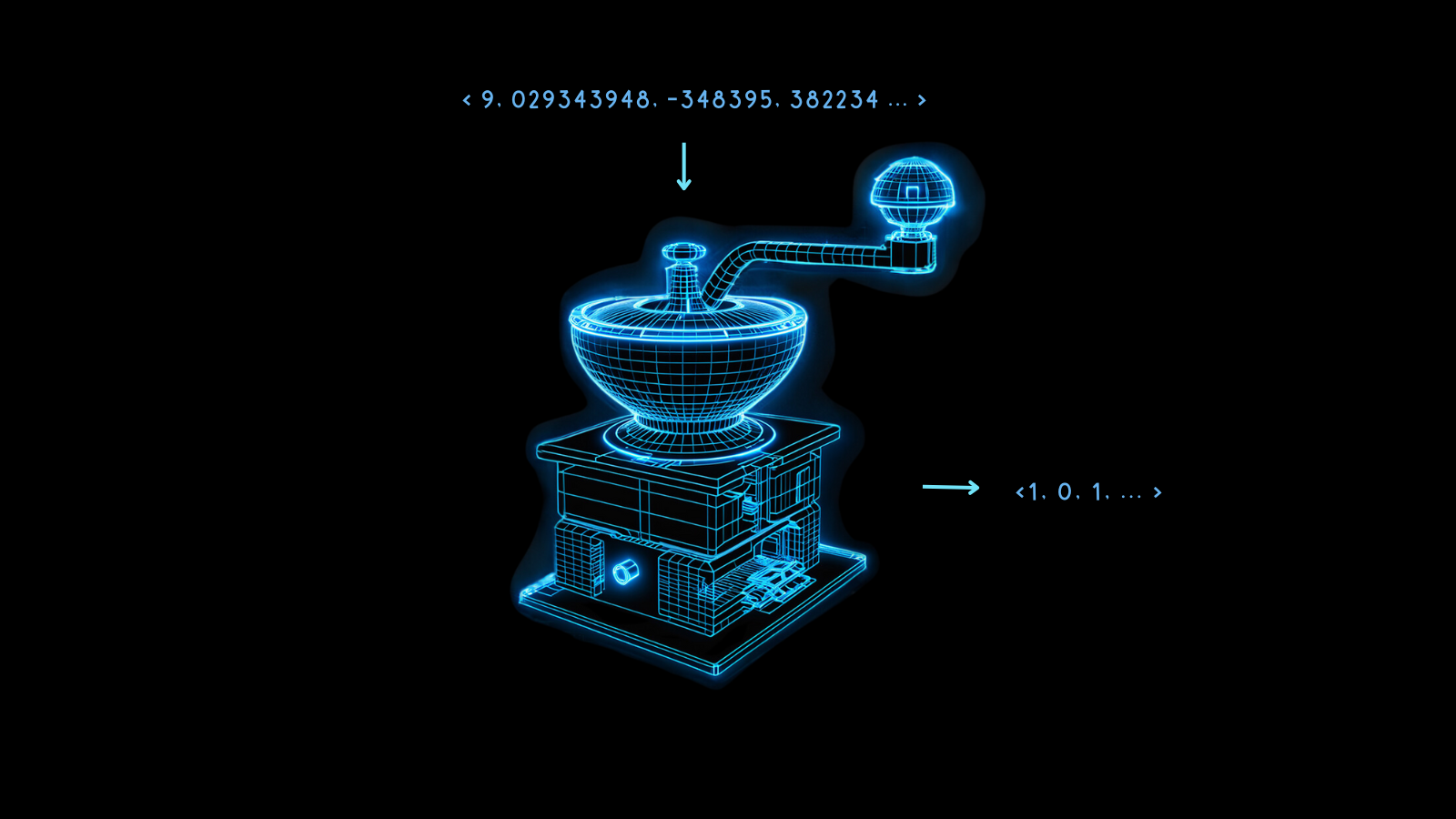
The magic behind binary embeddings is quantization, a method that turns high-precision numbers into lower-precision ones. In AI modeling, this often means converting the 32-bit floating-point numbers in embeddings into representations with fewer bits, like 8-bit integers.

Binary embeddings take this to its ultimate extreme, reducing each value to 0 or 1. Transforming 32-bit floating point numbers to binary digits cuts the size of embedding vectors 32-fold, a reduction of 96.875%. Vector operations on the resulting embeddings are much faster as a result. Using hardware speed-ups available on some microchips can increase the speed of vector comparisons by much more than 32-fold when the vectors are binarized.
Some information is inevitably lost during this process, but this loss is minimized when the model is very performant. If the non-quantized embeddings of different things are maximally different, then binarization is more likely to preserve that difference well. Otherwise, it can be difficult to interpret the embeddings correctly.
Jina Embeddings models are trained to be very robust in exactly that way, making them well-suited to binarization.
Such compact embeddings make new AI applications possible, particularly in resource-constrained contexts like mobile and time-sensitive uses.
These cost and computing time benefits come at a relatively small performance cost, as the chart below shows.

For jina-embeddings-v2-base-en, binary quantization reduces retrieval accuracy from 47.13% to 42.05%, a loss of approximately 10%. For jina-embeddings-v2-base-de, this loss is only 4%, from 44.39% to 42.65%.
Jina Embeddings models perform so well when producing binary vectors because they are trained to create a more uniform distribution of embeddings. This means that two different embeddings will likely be further from each other in more dimensions than embeddings from other models. This property ensures that those distances are better represented by their binary forms.
tagHow Do Binary Embeddings Work?
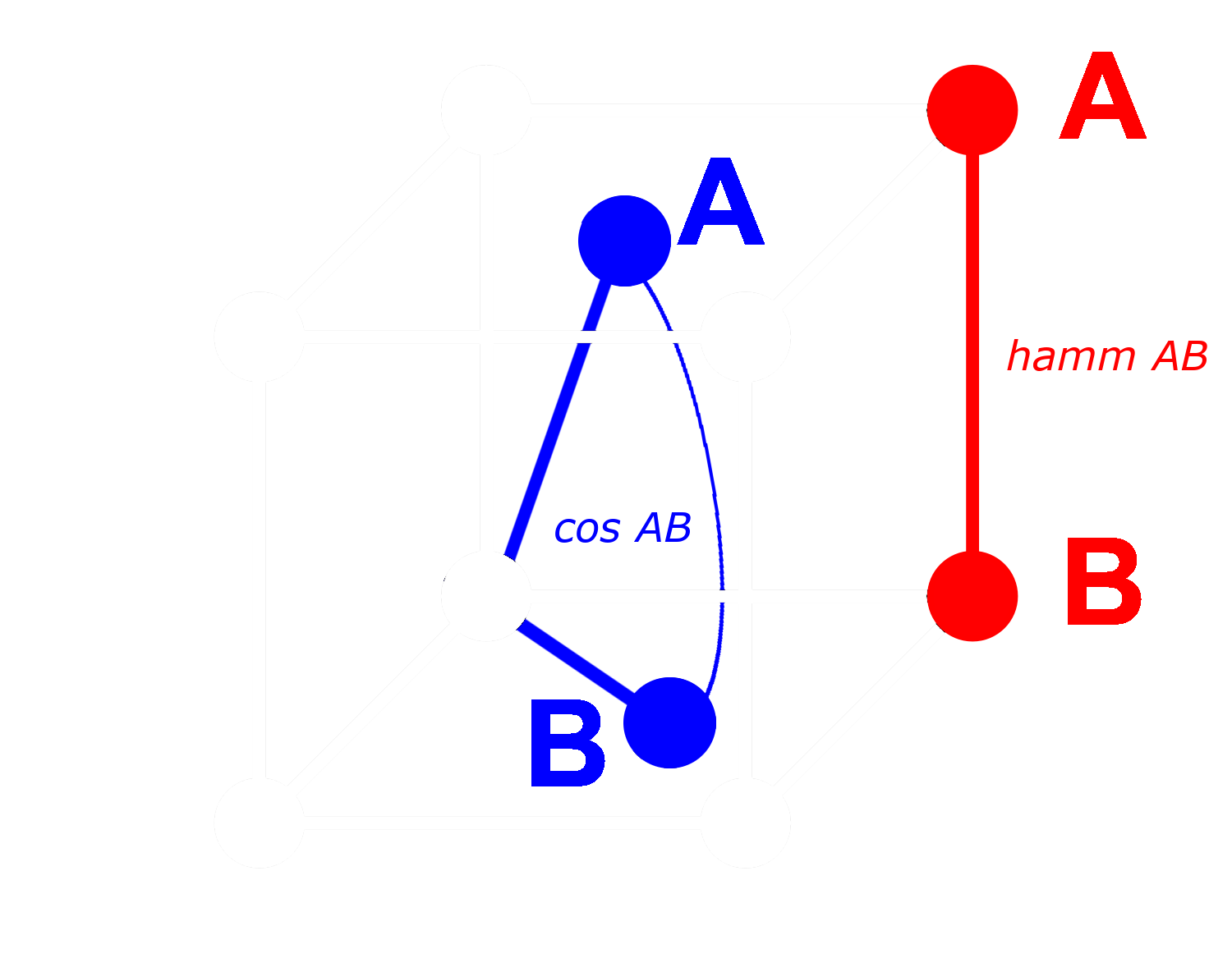
To see how this works, consider three embeddings: A, B, and C. These three are all full floating-point vectors, not binarized ones. Now, let’s say the distance from A to B is greater than the distance from B to C. With embeddings, we typically use the cosine distance, so:
If we binarize A, B, and C, we can measure distance more efficiently with Hamming distance.

Let’s call Abin, Bbin and Cbin the binarized versions of A, B and C.
For binary vectors, if the cosine distance between Abin and Bbin is greater than between Bbin and Cbin, then the Hamming distance between Abin and Bbin is greater than or equal to the Hamming distance between Bbin and Cbin.
So if:
then for Hamming distances:
Ideally, when we binarize embeddings, we want the same relationships with full embeddings to hold for the binary embeddings as for the full ones. This means that if one distance is greater than another for floating point cosine, it should be greater for the Hamming distance between their binarized equivalents:
We can’t make this true for all triplets of embeddings, but we can make it true for almost all of them.

With a binary vector, we can treat every dimension as either present (a one) or absent (a zero). The more distant two vectors are from each other in non-binary form, the higher the probability that in any one dimension, one will have a positive value and the other a negative value. This means that in binary form, there will most likely be more dimensions where one has a zero and the other a one. This makes them further apart by Hamming distance.
The opposite applies to vectors that are closer together: The closer the non-binary vectors are, the higher the probability that in any dimension both have zeros or both have ones. This makes them closer by Hamming distance.
Jina Embeddings models are so well-suited to binarization because we train them using negative mining and other fine-tuning practices to especially increase the distance between dissimilar things and reduce the distance between similar ones. This makes the embeddings more robust, more sensitive to similarities and differences, and makes the Hamming distance between binary embeddings more proportionate to the cosine distance between non-binary ones.
tagHow Much Can I Save with Jina AI's Binary Embeddings?
Embracing Jina AI’s binary embedding models doesn't just lower latency in time-sensitive applications, but also yields considerable cost benefits, as shown in the table below:
| Model | Memory per 250 million embeddings |
Retrieval benchmark average |
Estimated price on AWS ($3.8 per GB/month with x2gb instances) |
|---|---|---|---|
| 32-bit floating point embeddings | 715 GB | 47.13 | $35,021 |
| Binary embeddings | 22.3 GB | 42.05 | $1,095 |
This savings of over 95% is accompanied by only ~10% reduction in retrieval accuracy.
These are even greater savings than using binarized vectors from OpenAI's Ada 2 model or Cohere’s Embed v3, both of which produce output embeddings of 1024 dimensions or more. Jina AI’s embeddings have only 768 dimensions and still perform comparably to other models, making them smaller even before quantization for the same accuracy.
These savings are also environmental, using fewer rare materials and less energy.
tagGet Started
To get binary embeddings using the Jina Embeddings API, just add the parameter encoding_type to your API call, with the value binary to get the binarized embedding encoded as signed integers, or ubinary for unsigned integers.
tagDirectly Access Jina Embedding API
Using curl:
curl https://api.jina.ai/v1/embeddings \
-H "Content-Type: application/json" \
-H "Authorization: Bearer <YOUR API KEY>" \
-d '{
"input": ["Your text string goes here", "You can send multiple texts"],
"model": "jina-embeddings-v2-base-en",
"encoding_type": "binary"
}'
Or via the Python requests API:
import requests
headers = {
"Content-Type": "application/json",
"Authorization": "Bearer <YOUR API KEY>"
}
data = {
"input": ["Your text string goes here", "You can send multiple texts"],
"model": "jina-embeddings-v2-base-en",
"encoding_type": "binary",
}
response = requests.post(
"https://api.jina.ai/v1/embeddings",
headers=headers,
json=data,
)
With the above Python request, you will get the following response by inspecting response.json():
{
"model": "jina-embeddings-v2-base-en",
"object": "list",
"usage": {
"total_tokens": 14,
"prompt_tokens": 14
},
"data": [
{
"object": "embedding",
"index": 0,
"embedding": [
-0.14528547,
-1.0152762,
...
]
},
{
"object": "embedding",
"index": 1,
"embedding": [
-0.109809875,
-0.76077706,
...
]
}
]
}
These are two binary embedding vectors stored as 96 8-bit signed integers. To unpack them to 768 0’s and 1’s, you need to use the numpy library:
import numpy as np
# assign the first vector to embedding0
embedding0 = response.json()['data'][0]['embedding']
# convert embedding0 to a numpy array of unsigned 8-bit ints
uint8_embedding = np.array(embedding0).astype(numpy.uint8)
# unpack to binary
np.unpackbits(uint8_embedding)
The result is a 768-dimension vector with only 0’s and 1’s:
array([0, 0, 1, 1, 0, 1, 1, 0, 1, 1, 0, 0, 0, 1, 0, 1, 1, 1, 1, 1, 0, 0,
0, 0, 1, 1, 1, 1, 1, 1, 0, 0, 1, 1, 0, 0, 0, 1, 1, 1, 0, 1, 0, 1,
0, 0, 0, 0, 0, 0, 1, 0, 1, 0, 0, 1, 1, 0, 0, 0, 0, 1, 0, 1, 1, 1,
0, 0, 0, 0, 1, 1, 1, 0, 0, 1, 0, 0, 0, 0, 1, 1, 1, 1, 0, 1, 0, 1,
1, 1, 0, 1, 1, 1, 1, 0, 0, 0, 1, 1, 1, 1, 1, 0, 1, 0, 1, 0, 0, 0,
0, 0, 1, 0, 0, 0, 1, 0, 1, 1, 0, 0, 1, 0, 1, 1, 1, 1, 0, 0, 1, 0,
1, 0, 0, 1, 1, 0, 0, 1, 0, 1, 1, 0, 0, 0, 0, 1, 0, 0, 1, 0, 0, 1,
1, 0, 1, 0, 1, 1, 0, 0, 0, 1, 0, 1, 1, 1, 0, 0, 1, 1, 0, 0, 0, 1,
1, 1, 0, 1, 0, 1, 1, 1, 1, 0, 1, 0, 0, 1, 0, 0, 1, 0, 1, 0, 1, 1,
0, 0, 0, 1, 1, 1, 0, 0, 0, 0, 0, 0, 1, 1, 0, 1, 0, 0, 0, 1, 1, 1,
1, 0, 0, 1, 0, 0, 0, 1, 0, 1, 0, 0, 1, 0, 1, 0, 1, 0, 0, 1, 0, 0,
0, 0, 0, 0, 1, 0, 0, 0, 1, 1, 1, 0, 1, 1, 0, 1, 1, 0, 1, 0, 0, 0,
1, 0, 0, 1, 0, 0, 1, 0, 0, 0, 1, 1, 0, 1, 1, 0, 0, 0, 1, 0, 0, 1,
0, 0, 0, 0, 0, 1, 1, 0, 0, 1, 1, 1, 1, 0, 1, 0, 1, 0, 1, 1, 1, 1,
1, 0, 1, 0, 0, 0, 1, 0, 0, 1, 0, 1, 1, 1, 0, 1, 1, 1, 1, 1, 1, 0,
0, 0, 0, 0, 1, 0, 1, 1, 1, 0, 1, 1, 1, 1, 0, 0, 0, 0, 0, 1, 1, 1,
1, 1, 1, 1, 0, 1, 0, 0, 0, 0, 0, 0, 1, 0, 0, 1, 0, 1, 0, 1, 0, 1,
1, 0, 1, 1, 1, 0, 0, 1, 0, 1, 1, 0, 1, 0, 0, 1, 1, 0, 0, 0, 1, 1,
0, 0, 0, 1, 1, 1, 1, 1, 0, 1, 1, 0, 1, 0, 0, 0, 1, 1, 0, 1, 1, 0,
1, 0, 1, 0, 0, 0, 0, 0, 0, 1, 0, 0, 0, 1, 1, 1, 1, 0, 1, 1, 1, 0,
0, 0, 0, 0, 0, 1, 1, 1, 1, 0, 1, 0, 1, 1, 0, 1, 0, 1, 1, 1, 0, 0,
0, 0, 1, 1, 1, 0, 1, 0, 1, 0, 0, 1, 0, 1, 0, 0, 0, 1, 1, 1, 0, 1,
0, 1, 1, 1, 0, 1, 1, 0, 1, 0, 1, 1, 1, 1, 1, 0, 1, 0, 0, 0, 1, 0,
0, 1, 1, 1, 0, 1, 1, 0, 0, 1, 1, 0, 1, 1, 0, 1, 1, 1, 0, 1, 1, 0,
1, 1, 0, 1, 0, 0, 0, 0, 0, 1, 0, 0, 0, 0, 1, 1, 1, 1, 0, 1, 1, 0,
0, 1, 0, 0, 1, 1, 0, 1, 0, 0, 1, 0, 0, 1, 0, 1, 0, 1, 1, 1, 0, 0,
0, 0, 1, 1, 0, 1, 0, 0, 1, 1, 1, 1, 1, 0, 1, 0, 1, 1, 1, 1, 0, 1,
1, 0, 1, 1, 0, 1, 1, 0, 1, 0, 0, 1, 0, 0, 0, 1, 0, 1, 0, 1, 1, 0,
1, 1, 1, 0, 0, 0, 1, 0, 0, 1, 0, 0, 0, 1, 0, 0, 1, 0, 1, 1, 0, 0,
1, 0, 1, 1, 1, 1, 1, 1, 1, 0, 1, 0, 0, 0, 1, 0, 0, 1, 1, 1, 0, 1,
1, 1, 0, 1, 0, 0, 0, 0, 0, 1, 0, 0, 1, 1, 0, 1, 1, 0, 0, 1, 1, 0,
1, 0, 1, 0, 0, 0, 0, 0, 0, 0, 1, 1, 0, 0, 0, 1, 0, 0, 1, 1, 0, 1,
1, 1, 1, 0, 0, 1, 1, 1, 0, 1, 0, 0, 1, 1, 0, 1, 1, 1, 1, 1, 1, 0,
1, 1, 1, 0, 0, 1, 1, 0, 0, 1, 0, 0, 1, 1, 0, 0, 0, 1, 0, 1, 1, 1,
0, 0, 1, 1, 0, 0, 1, 0, 1, 1, 1, 1, 1, 0, 1, 0, 0, 1, 0, 0],
dtype=uint8)
tagUsing Binary Quantization in Qdrant
You can also use Qdrant's integration library to put binary embeddings directly in your Qdrant vector store. As Qdrant has internally implemented BinaryQuantization, you can use it as a preset configuration for the entire vector collection, making it retrieve and store binary vectors without any other changes to your code.
See the example code below for how:
import qdrant_client
import requests
from qdrant_client.models import Distance, VectorParams, Batch, BinaryQuantization, BinaryQuantizationConfig
# Provide Jina API key and choose one of the available models.
# You can get a free trial key here: https://jina.ai/embeddings/
JINA_API_KEY = "jina_xxx"
MODEL = "jina-embeddings-v2-base-en" # or "jina-embeddings-v2-base-en"
EMBEDDING_SIZE = 768 # 512 for small variant
# Get embeddings from the API
url = "https://api.jina.ai/v1/embeddings"
headers = {
"Content-Type": "application/json",
"Authorization": f"Bearer {JINA_API_KEY}",
}
text_to_encode = ["Your text string goes here", "You can send multiple texts"]
data = {
"input": text_to_encode,
"model": MODEL,
}
response = requests.post(url, headers=headers, json=data)
embeddings = [d["embedding"] for d in response.json()["data"]]
# Index the embeddings into Qdrant
client = qdrant_client.QdrantClient(":memory:")
client.create_collection(
collection_name="MyCollection",
vectors_config=VectorParams(size=EMBEDDING_SIZE, distance=Distance.DOT, on_disk=True),
quantization_config=BinaryQuantization(binary=BinaryQuantizationConfig(always_ram=True)),
)
client.upload_collection(
collection_name="MyCollection",
ids=list(range(len(embeddings))),
vectors=embeddings,
payload=[
{"text": x} for x in text_to_encode
],
)To configure for search, you should use the oversampling and rescore parameters:
from qdrant_client.models import SearchParams, QuantizationSearchParams
results = client.search(
collection_name="MyCollection",
query_vector=embeddings[0],
search_params=SearchParams(
quantization=QuantizationSearchParams(
ignore=False,
rescore=True,
oversampling=2.0,
)
)
)tagUsing LlamaIndex
To use Jina binary embeddings with LlamaIndex, set the encoding_queries parameter to binary when instantiating theJinaEmbedding object:
from llama_index.embeddings.jinaai import JinaEmbedding
# You can get a free trial key from https://jina.ai/embeddings/
JINA_API_KEY = "<YOUR API KEY>"
jina_embedding_model = JinaEmbedding(
api_key=jina_ai_api_key,
model="jina-embeddings-v2-base-en",
encoding_queries='binary',
encoding_documents='float'
)
jina_embedding_model.get_query_embedding('Query text here')
jina_embedding_model.get_text_embedding_batch(['X', 'Y', 'Z'])
tagOther Vector Databases Supporting Binary Embeddings
The following vector databases provide native support for binary vectors:
tagExample
To show you binary embeddings in action, we took a selection of abstracts from arXiv.org, and got both 32-bit floating point and binary vectors for them using jina-embeddings-v2-base-en. We then compared them to the embeddings for an example query: "3D segmentation."
You can see from the table below that the top three answers are the same and four of the top five match. Using binary vectors produces almost identical top matches.
| Binary | 32-bit Float | |||
|---|---|---|---|---|
| Rank | Hamming dist. |
Matching Text | Cosine | Matching text |
| 1 | 0.1862 | SEGMENT3D: A Web-based Application for Collaboration... |
0.2340 | SEGMENT3D: A Web-based Application for Collaboration... |
| 2 | 0.2148 | Segmentation-by-Detection: A Cascade Network for... |
0.2857 | Segmentation-by-Detection: A Cascade Network for... |
| 3 | 0.2174 | Vox2Vox: 3D-GAN for Brain Tumour Segmentation... |
0.2973 | Vox2Vox: 3D-GAN for Brain Tumour Segmentation... |
| 4 | 0.2318 | DiNTS: Differentiable Neural Network Topology Search... |
0.2983 | Anisotropic Mesh Adaptation for Image Segmentation... |
| 5 | 0.2331 | Data-Driven Segmentation of Post-mortem Iris Image... |
0.3019 | DiNTS: Differentiable Neural Network Topology... |


