Does Subspace Cosine Similarity Imply High-Dimensional Cosine Similarity?

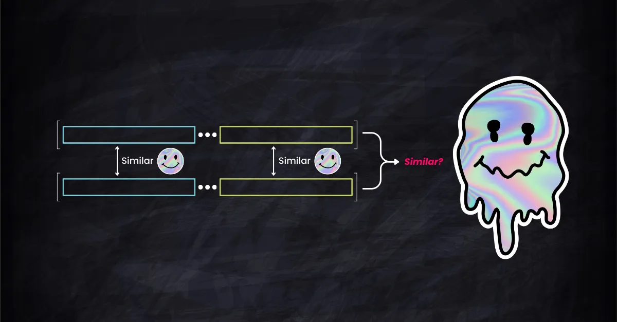
Consider this: when measuring the cosine similarity of embedding vectors in high-dimensional spaces, how does their similarity in lower-dimensional subspaces imply the overall similarity? Is there a direct, proportional relationship, or is the reality more complex with high-dimensional data?

More concretely, does high similarity between vectors in their first 256 dimensions assure a high similarity in their full 768 dimensions? Conversely, if vectors significantly differ in some dimensions, does this spell a low overall similarity? These aren't mere theoretical musings; they are crucial considerations for efficient vector retrieval, database indexing, and the performance of RAG systems.

Developers often rely on heuristics, assuming that high subspace similarity equates to high overall similarity or that notable differences in one dimension significantly affect the overall similarity. The question is: are these heuristic methods built on firm theoretical ground, or are they simply assumptions of convenience?

This post delves into these questions, examining the theory and practical implications of subspace similarity in relation to overall vector similarity.

tagBounding the Cosine Similarity

Given vectors $\mathbf{A}, \mathbf{B}\in \mathbb{R}^d$, we decompose them as $\mathbf{A}=[\mathbf{A}_1, \mathbf{A}_2]$ and $\mathbf{B}=[\mathbf{B}_1, \mathbf{B}_2]$, where $\mathbf{A}_1,\mathbf{B}_1\in\mathbb{R}^m$ and $\mathbf{A}_2,\mathbf{B}_2\in\mathbb{R}^n$, with $m+n=d$.

The cosine similarity in the subspace $\mathbb{R}^m$ is given by $\cos(\mathbf{A}_1, \mathbf{B}_1)=\frac{\mathbf{A}_1\cdot\mathbf{B}_1}{\|\mathbf{A}_1\|\|\mathbf{B}_1\|}$; similarly, the similarity in the subspace $\mathbb{R}^n$ is $\cos(\mathbf{A}_2, \mathbf{B}_2)=\frac{\mathbf{A}_2\cdot\mathbf{B}_2}{\|\mathbf{A}_2\|\|\mathbf{B}_2\|}$.

In the original space $\mathbb{R}^d$, the cosine similarity is defined as:$$\begin{align*}\cos(\mathbf{A},\mathbf{B})&=\frac{\mathbf{A}\cdot\mathbf{B}}{\|\mathbf{A}\|\|\mathbf{B}\|}\\&=\frac{\mathbf{A}_1\cdot\mathbf{B}_1+\mathbf{A}_2\cdot\mathbf{B}_2}{\sqrt{\|\mathbf{A}_1\|^2+\|\mathbf{A}_2\|^2}\sqrt{\|\mathbf{B}_1\|^2+\|\mathbf{B}_2\|^2}}\\&=\frac{\cos(\mathbf{A}_1, \mathbf{B}_1)\|\mathbf{A}_1\|\|\mathbf{B}_1\|+\cos(\mathbf{A}_2, \mathbf{B}_2)\|\mathbf{A}_2\|\|\mathbf{B}_2\|}{\sqrt{\|\mathbf{A}_1\|^2+\|\mathbf{A}_2\|^2}\sqrt{\|\mathbf{B}_1\|^2+\|\mathbf{B}_2\|^2}}\end{align*}$$

Now, let $s := \max(\cos(\mathbf{A}_1, \mathbf{B}_1), \cos(\mathbf{A}_2, \mathbf{B}_2))$. Then, we have:$$\begin{align*}\cos(\mathbf{A},\mathbf{B})&\leq\frac{s\|\mathbf{A}_1\|\|\mathbf{B}_1\|+s\|\mathbf{A}_2\|\|\mathbf{B}_2\|}{\sqrt{\|\mathbf{A}_1\|^2+\|\mathbf{A}_2\|^2}\sqrt{\|\mathbf{B}_1\|^2+\|\mathbf{B}_2\|^2}}\\&=\frac{\|\mathbf{A}_1\|\|\mathbf{B}_1\|+\|\mathbf{A}_2\|\|\mathbf{B}_2\|}{\sqrt{\|\mathbf{A}_1\|^2+\|\mathbf{A}_2\|^2}\sqrt{\|\mathbf{B}_1\|^2+\|\mathbf{B}_2\|^2}}\cdot s\\&=\cos(\underbrace{[\|\mathbf{A}_1\|, \|\mathbf{A}_2\|]}_{\mathbb{R}^2}, \underbrace{[\|\mathbf{B}_1\|, \|\mathbf{B}_2\|]}_{\mathbb{R}^2})\cdot s\\&\leq 1\cdot s \\&= \max(\cos(\mathbf{A}_1, \mathbf{B}_1), \cos(\mathbf{A}_2, \mathbf{B}_2))\end{align*}$$

End of proof.

Note that in the final step of the proof, we leverage that the cosine similarity is always less than or equal to 1. This forms our upper bound. Similarly, we can show that the lower bound of $\cos(\mathbf{A},\mathbf{B})$ is given by:

$$\cos(\mathbf{A},\mathbf{B}) \geq t \cdot \cos([\|\mathbf{A}_1\|, \|\mathbf{A}_2\|], [\|\mathbf{B}_1\|, \|\mathbf{B}_2\|])$$, where $t:= \min(\cos(\mathbf{A}_1, \mathbf{B}_1), \cos(\mathbf{A}_2, \mathbf{B}_2))$.

Note that for the lower bound, we can not hastily conclude that $\cos(\mathbf{A},\mathbf{B}) \geq t$. This is because of the range of the cosine function, which spans between $[-1, 1]$. Due to this range, it's impossible to establish a tighter lower bound than the trivial value of -1.

So in conclusion, we have the following loose bound: $$-1\leq\cos(\mathbf{A},\mathbf{B})\leq\max(\cos(\mathbf{A}_1, \mathbf{B}_1), \cos(\mathbf{A}_2, \mathbf{B}_2)).$$ and a tighter bound $$\begin{align*} \gamma \cdot t\leq&\cos(\mathbf{A}, \mathbf{B}) \leq\gamma\cdot s\\\gamma \cdot \min(\cos(\mathbf{A}_1, \mathbf{B}_1), \cos(\mathbf{A}_2, \mathbf{B}_2)) \leq &\cos(\mathbf{A}, \mathbf{B}) \leq \gamma \cdot \max(\cos(\mathbf{A}_1, \mathbf{B}_1), \cos(\mathbf{A}_2, \mathbf{B}_2))\end{align*}$$, where $\gamma = \cos([\|\mathbf{A}_1\|, \|\mathbf{A}_2\|], [\|\mathbf{B}_1\|, \|\mathbf{B}_2\|])$.

tagConnection to Johnson–Lindenstrauss Lemma

The JL lemma asserts that for any $0 < \epsilon < 1$ and any finite set of points $S$ in $\mathbb{R}^d$, there exists a mapping $f: \mathbb{R}^d \rightarrow \mathbb{R}^k$ (with $k = O(\epsilon^{-2} \log |S|)$) such that for all $\mathbf{u}, \mathbf{v} \in S$, the Euclidean distances are approximately preserved:

$$(1 - \epsilon) \|\mathbf{u} - \mathbf{v}\|^2 \leq \|f(\mathbf{u}) - f(\mathbf{v})\|^2 \leq (1 + \epsilon) \|\mathbf{u} - \mathbf{v}\|^2$$

Johnson–Lindenstrauss lemma - Wikipedia

Wikimedia Foundation, Inc.Contributors to Wikimedia projects

To make $f$ work like a subspace selection, we can use a diagonal matrix for projection, such as a $5 \times 3$ matrix $f$, albeit not random (note, the typical formulation of the JL lemma involves linear transformations that often utilize random matrices drawn from a Gaussian distribution). For instance, if we aim to retain the 1st, 3rd, and 5th dimensions from a 5-dimensional vector space, the matrix $f$ could be designed as follows: $$f = \begin{bmatrix}1 & 0 & 0 \\0 & 0 & 0 \\0 & 1 & 0 \\0 & 0 & 0 \\0 & 0 & 1\end{bmatrix}$$
However, by specifying $f$ to be diagonal, we limit the class of functions that can be used for the projection. The JL lemma guarantees the existence of a suitable $f$ within the broader class of linear transformations, but when we restrict $f$ to be diagonal, such a suitable $f$ may not exist within this restricted class for applying the JL lemma's bounds.

tagValidating the Bounds

To empirically explore the theoretical bounds on cosine similarity in high-dimensional vector spaces, we can employ a Monte Carlo simulation. This method allows us to generate a large number of random vector pairs, compute their similarities in both the original space and subspaces, and then assess how well the theoretical upper and lower bounds hold in practice.

The following Python code snippet implements this concept. It randomly generates pairs of vectors in a high-dimensional space and computes their cosine similarity. Then, it divides each vector into two subspaces, calculates the cosine similarity within each subspace, and evaluates the upper and lower bounds of the full-dimensional cosine similarity based on the subspace similarities.

import numpy as np


def compute_cosine_similarity(U, V):
    # Normalize the rows to unit vectors
    U_norm = U / np.linalg.norm(U, axis=1, keepdims=True)
    V_norm = V / np.linalg.norm(V, axis=1, keepdims=True)
    # Compute pairwise cosine similarity
    return np.sum(U_norm * V_norm, axis=1)


# Generate random data
num_points = 5000
d = 1024
A = np.random.random([num_points, d])
B = np.random.random([num_points, d])

# Compute cosine similarity between A and B
cos_sim = compute_cosine_similarity(A, B)

# randomly divide A and B into subspaces
m = np.random.randint(1, d)
A1 = A[:, :m]
A2 = A[:, m:]
B1 = B[:, :m]
B2 = B[:, m:]

# Compute cosine similarity in subspaces
cos_sim1 = compute_cosine_similarity(A1, B1)
cos_sim2 = compute_cosine_similarity(A2, B2)

# Find the element-wise maximum and minimum of cos_sim1 and cos_sim2
s = np.maximum(cos_sim1, cos_sim2)
t = np.minimum(cos_sim1, cos_sim2)

norm_A1 = np.linalg.norm(A1, axis=1)
norm_A2 = np.linalg.norm(A2, axis=1)
norm_B1 = np.linalg.norm(B1, axis=1)
norm_B2 = np.linalg.norm(B2, axis=1)

# Form new vectors in R^2 from the norms
norm_A_vectors = np.stack((norm_A1, norm_A2), axis=1)
norm_B_vectors = np.stack((norm_B1, norm_B2), axis=1)

# Compute cosine similarity in R^2
gamma = compute_cosine_similarity(norm_A_vectors, norm_B_vectors)

# print some info and validate the lower bound and upper bound
print('d: %d\n'
      'm: %d\n'
      'n: %d\n'
      'avg. cosine(A,B): %f\n'
      'avg. upper bound: %f\n'
      'avg. lower bound: %f\n'
      'lower bound satisfied: %s\n'
      'upper bound satisfied: %s' % (
          d, m, (d - m), np.mean(cos_sim), np.mean(s), np.mean(gamma * t), np.all(s >= cos_sim),
          np.all(gamma * t <= cos_sim)))
Copy

d: 1024
m: 743
n: 281
avg. cosine(A,B): 0.750096
avg. upper bound: 0.759080
avg. lower bound: 0.741200
lower bound satisfied: True
upper bound satisfied: True

tagUnderstanding the Bounds

In a nutshell, when comparing two high-dimensional vectors, the overall similarity lies between the best and worst similarities of their subspaces, adjusted for how large or important those subspaces are in the overall scheme. This is what the bounds for cosine similarity in higher dimensions intuitively represent: the balance between the most and least similar parts, weighted by their relative sizes or importance.

Imagine you're trying to compare two multi-part objects (let's say, two fancy pens) based on their overall similarity. Each pen has two main components: the body and the cap. The similarity of the whole pen (both body and cap) is what we're trying to determine:

tagUpper Bound ($\gamma \cdot s$)

Think of $s$ as the best match between corresponding parts of the pens. If the caps are very similar but the bodies aren't, $s$ is the similarity of the caps.

Now, $\gamma$ is like a scaling factor based on the size (or importance) of each part. If one pen has a very long body and a short cap, while the other has a short body and a long cap, $\gamma$ adjusts the overall similarity to account for these differences in proportions.

The upper bound tells us that no matter how similar some parts are, the overall similarity can't exceed this "best part similarity" scaled by the proportion factor.

tagLower Bound ($\gamma \cdot t$)

Here, $t$ is the similarity of the least matching parts. If the bodies of the pens are quite different but the caps are similar, $t$ reflects the body's similarity.

Again, $\gamma$ scales this based on the proportion of each part.

The lower bound means that the overall similarity can't be worse than this "worst part similarity" after accounting for the proportion of each part.

tagImplications of the Bounds

For software engineers working with embeddings, vector search, retrieval, or databases, understanding these bounds has practical implications, particularly when dealing with high-dimensional data. Vector search often involves finding the closest (most similar) vectors in a database to a given query vector, typically using cosine similarity as a measure of closeness. The bounds we discussed can provide insights into the effectiveness and limitations of using subspace similarities for such tasks.

tagUsing Subspace Similarity for Ranking

Safety and Accuracy: Using subspace similarity for ranking and retrieving top-k results can be effective, but with caution. The upper bound indicates that the overall similarity can't exceed the maximum similarity of the subspaces. Thus, if a pair of vectors is highly similar in a particular subspace, it's a strong candidate for being similar in the high-dimensional space.

Potential Pitfalls: However, the lower bound suggests that two vectors with low similarity in one subspace could still be quite similar overall. Therefore, relying solely on subspace similarity might miss some relevant results.

tagMisconceptions and Cautions

Overestimating Subspace Importance: A common misconception is overestimating the importance of a particular subspace. While high similarity in one subspace is a good indicator, it doesn't guarantee high overall similarity due to the influence of other subspaces.

Ignoring Negative Similarities: In cases where the cosine similarity in a subspace is negative, it indicates an opposing relationship in that dimension. Engineers should be wary of how these negative similarities impact the overall similarity.