Recently, Christoph Schuhmann, Founder of LAION AI shared an interesting observation about text embedding models:
When words within a sentence are randomly shuffled, the cosine similarity between their text embeddings remains surprisingly high compared to the original sentence.
For example, let's look at two sentences: Berlin is the capital of Germany and the Germany Berlin is capital of. Even though the second sentence makes no sense, text embedding models can't really tell them apart. Using jina-embeddings-v3, these two sentences have a cosine similarity score of 0.9295.
Word order isn’t the only thing for which embeddings seem not to be very sensitive. Grammatical transformations can dramatically change a sentence's meaning but have little impact on embedding distance. For example, She ate dinner before watching the movie and She watched the movie before eating dinner have a cosine similarity of 0.9833, despite having the opposite order of actions.
Negation is also notoriously difficult to embed consistently without special training — This is a useful model and This is not a useful model look practically the same in embedding space. Often, replacing the words in a text with others of the same class, like changing “today” to “yesterday”, or altering a verb tense, doesn’t change the embeddings as much as you might think it should.
This has serious implications. Consider two search queries: Flight from Berlin to Amsterdam and Flight from Amsterdam to Berlin. They have almost identical embeddings, with jina-embeddings-v3 assigning them a cosine similarity of 0.9884. For a real-world application like travel search or logistics, this shortcoming is fatal.
In this article, we look at challenges facing embedding models, examining their persistent struggles with word order and word choice. We analyze key failure modes across linguistic categories—including directional, temporal, causal, comparative, and negational contexts—while exploring strategies to enhance model performance.
tagWhy Do Shuffled Sentences Have Surprisingly Close Cosine Scores?
At first, we thought this might be down to how the model combines word meanings - it creates an embedding for each word (6-7 words in each of our example sentences above) and then averages these embeddings together with mean pooling. This means very little word order information is available to the final embedding. An average is the same no matter what order the values are in.
However, even models that use CLS pooling (which looks at a special first word to understand the whole sentence and should be more sensitive to word order) have the same problem. For example, bge-1.5-base-en still gives a cosine similarity score of 0.9304 for the sentences Berlin is the capital of Germany and the Germany Berlin is capital of.
This points to a limitation in how embedding models are trained. While language models initially learn sentence structure during pre-training, they seem to lose some of this understanding during contrastive training — the process we use to create embedding models.
tagHow do Text Length and Word Order Impact Embedding Similarity?
Why do models have trouble with word order in the first place? The first thing that comes to mind is the length (in tokens) of the text. When text is sent to the encoding function, the model first generates a list of token embeddings (i.e., each tokenized word has a dedicated vector representing its meaning), then averages them.
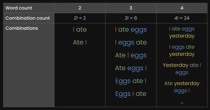
To see how text length and word order impact embedding similarity, we generated a dataset of 180 synthetic sentences of varying lengths, such as 3, 5, 10, 15, 20, and 30 tokens. We also randomly shuffled the tokens to form a variation of each sentence:
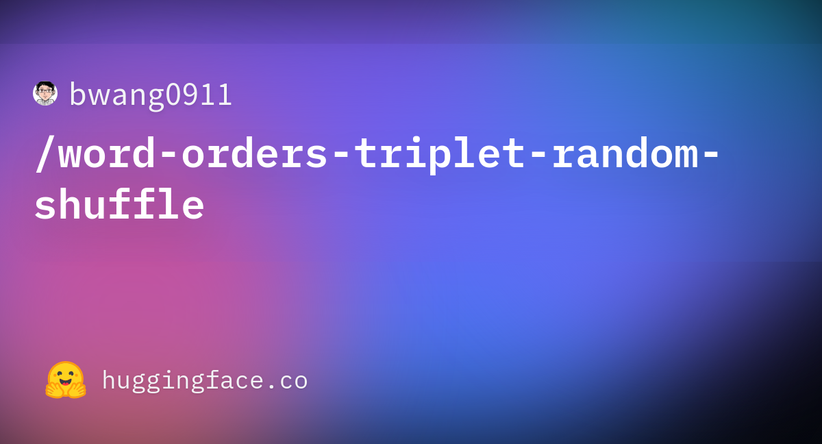
Here are a few examples:
| Length (tokens) | Original sentence | Shuffled sentence |
|---|---|---|
| 3 | The cat sleeps | cat The sleeps |
| 5 | He drives his car carefully | drives car his carefully He |
| 15 | The talented musicians performed beautiful classical music at the grand concert hall yesterday | in talented now grand classical yesterday The performed musicians at hall concert the music |
| 30 | The passionate group of educational experts collaboratively designed and implemented innovative teaching methodologies to improve learning outcomes in diverse classroom environments worldwide | group teaching through implemented collaboratively outcomes of methodologies across worldwide diverse with passionate and in experts educational classroom for environments now by learning to at improve from innovative The designed |
We’ll encode the dataset using our own jina-embeddings-v3 model and the open-source model bge-base-en-v1.5, then compute the cosine similarity between the original and the shuffled sentence:
| Length (tokens) | Mean cosine similarity | Standard deviation in cosine similarity |
|---|---|---|
| 3 | 0.947 | 0.053 |
| 5 | 0.909 | 0.052 |
| 10 | 0.924 | 0.031 |
| 15 | 0.918 | 0.019 |
| 20 | 0.899 | 0.021 |
| 30 | 0.874 | 0.025 |
We can now generate a box plot, which makes the trend in cosine similarity clearer:
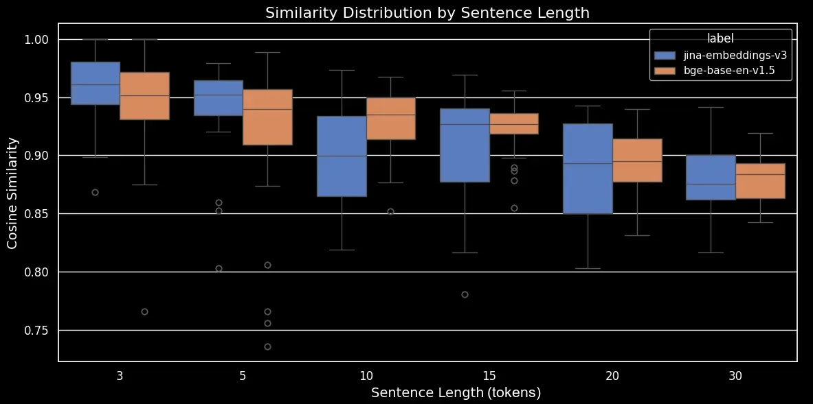
bge-base-en-1.5 (unfinetuned)As we can see, there’s a clear linear relationship in the average cosine similarity of embeddings. The longer the text, the lower the average cosine similarity score between the original and randomly shuffled sentences. This likely happens due to “word displacement”, namely, how far word have moved from their original positions after random shuffling. In a shorter text, there are simply fewer “slots” for a token to be shuffled to so it can’t move so far, while a longer text has a greater number of potential permutations and words can move a greater distance.
As shown in the figure below (Cosine Similarity vs Average Word Displacement), the longer the text, the greater the word displacement:
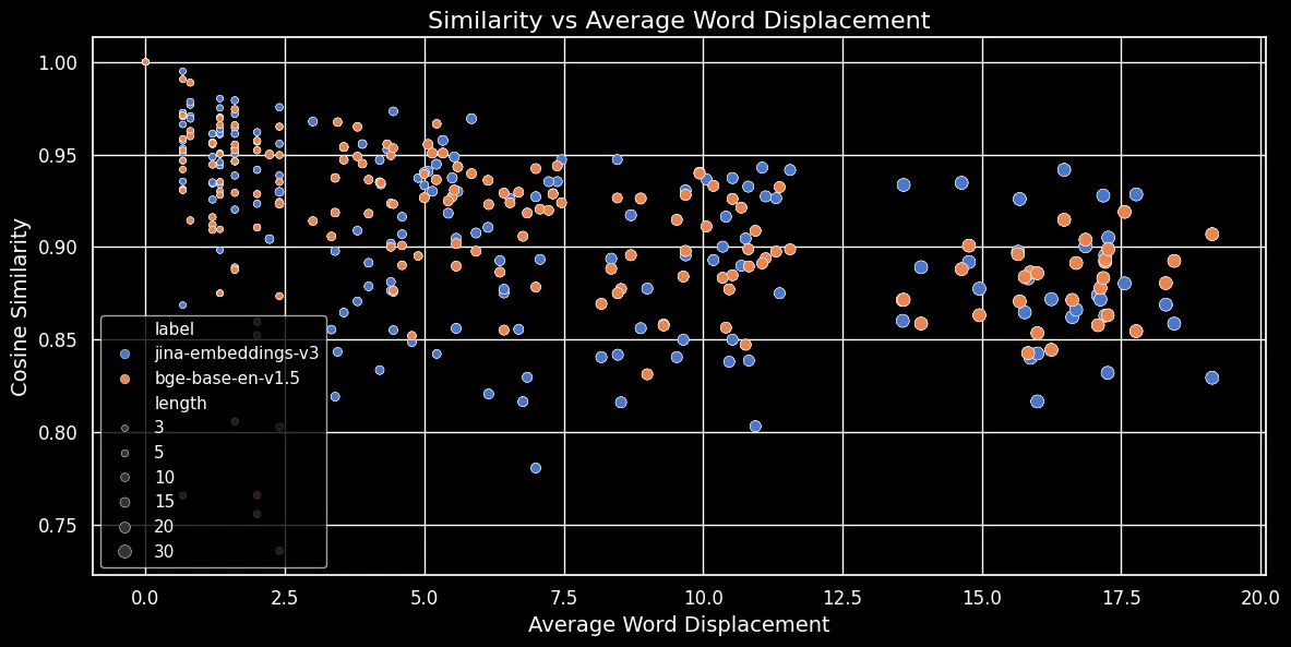
Token embeddings are dependent on local context, i.e. the words nearest to them. In a short text, rearranging words can’t change that context very much. However, for a longer text, a word might be moved very far away from its original context and that can change its token embedding quite a lot. As a result, shuffling the words in a longer text produces a more distant embedding than for a shorter one. The figure above shows that for both jina-embeddings-v3, using mean pooling, and bge-base-en-v1.5, using CLS pooling, the same relationship holds: Shuffling longer texts and displacing words farther results in smaller similarity scores.
tagDo Bigger Models Solve the Problem?
Usually, when we face this kind of problem, a common tactic is to just throw a bigger model at it. But can a larger text embedding model really capture word order information more effectively? According to the scaling law of text embedding models (referenced in our jina-embeddings-v3 release post), larger models generally provide better performance:
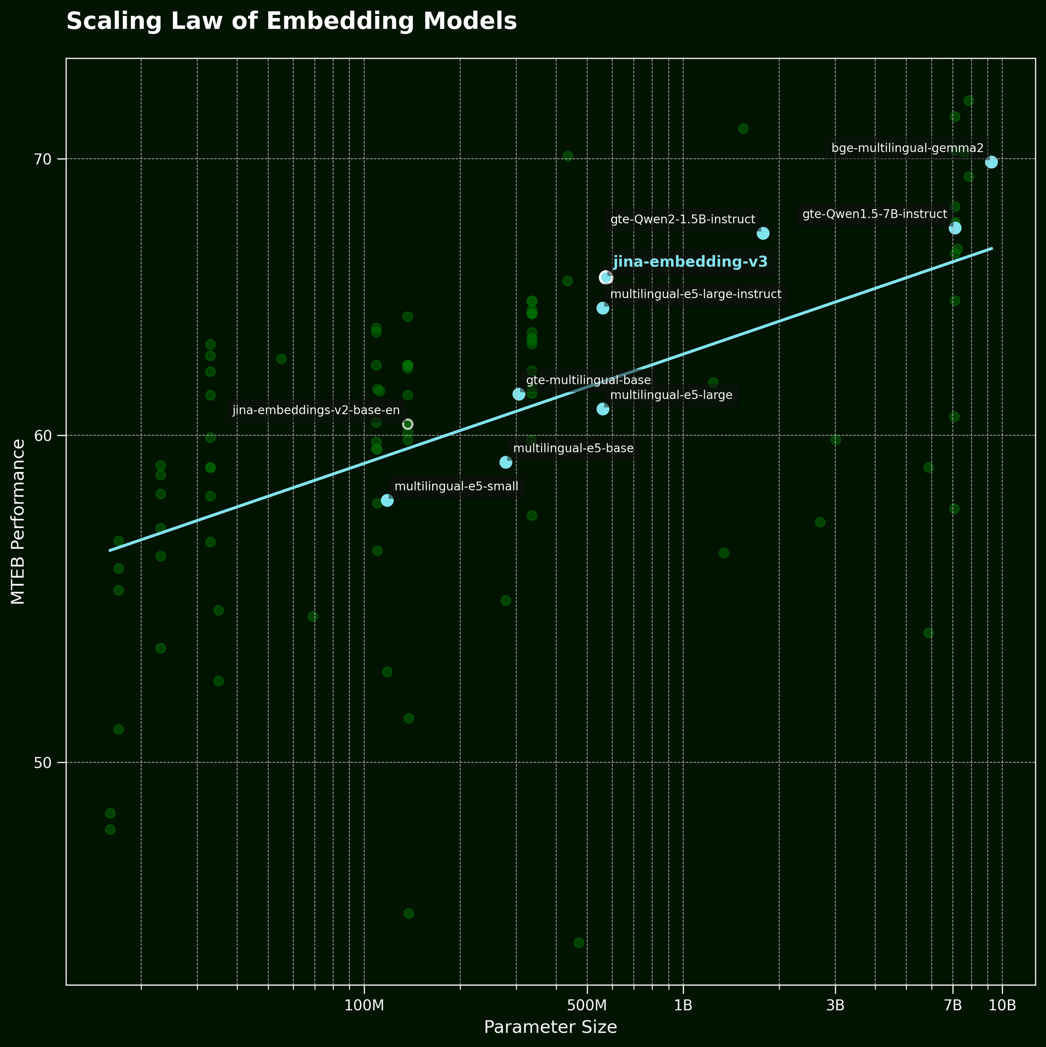
But can a larger model capture word order information more effectively? We tested three variations of the BGE model: bge-small-en-v1.5, bge-base-en-v1.5, and bge-large-en-v1.5, with parameter sizes of 33 million, 110 million, and 335 million, respectively.
We’ll use the same 180 sentences as before, but disregard the length information. We’ll encode both the original sentences and their random shuffles using the three model variants and plot the average cosine similarity:
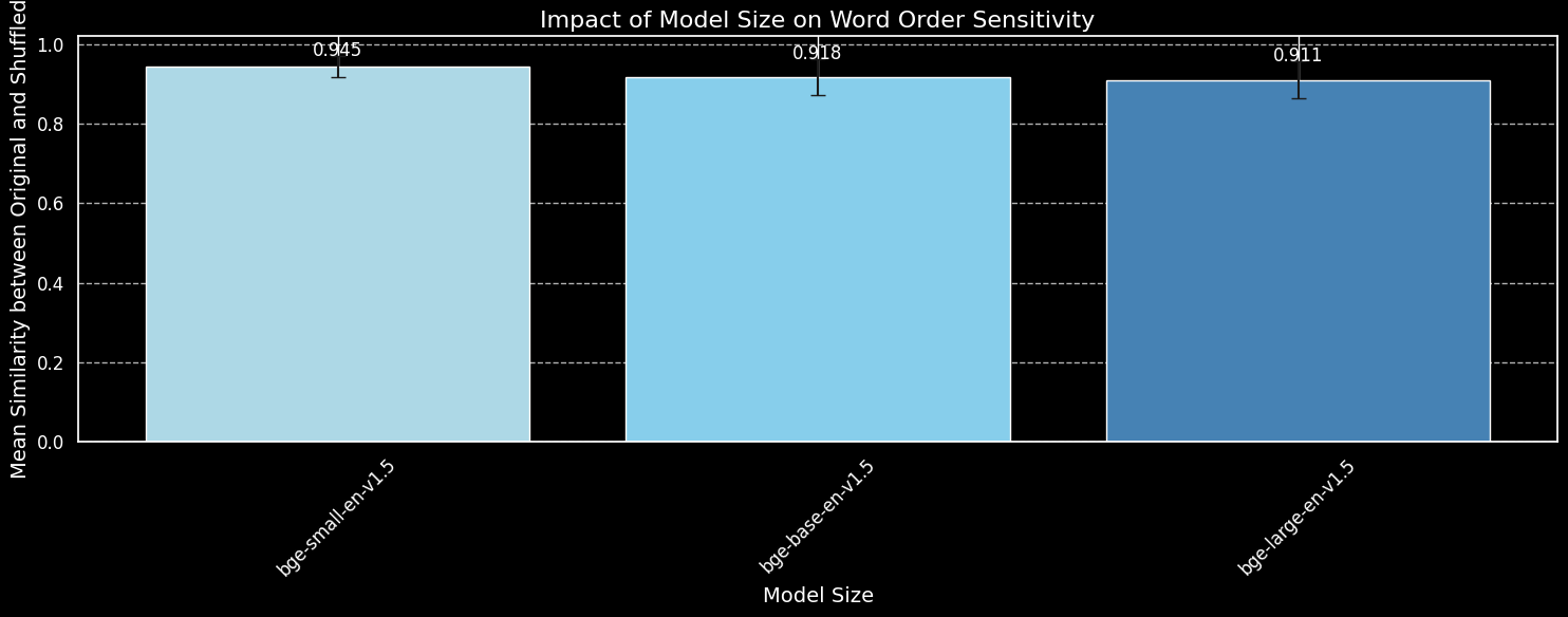
bge-small-en-v1.5, bge-base-en-v1.5, and bge-large-en-v1.5.While we can see that larger models are more sensitive to word order variation, the difference is small. Even the massively larger bge-large-en-v1.5 is at most a tiny bit better at distinguishing shuffled sentences from unshuffled ones. Other factors come into play in determining how sensitive an embedding model is to word reorderings, particularly differences in training regimen. Furthermore, cosine similarity is a very limited tool for measuring a model’s ability to make distinctions. However, we can see that model size is not a major consideration. We can’t simply make our model bigger and solve this problem.
tagWord Order and Word Choice in The Real World
jina-embeddings-v2 (not our most recent model, jina-embeddings-v3) since v2 is much smaller and thus faster to experiment with on our local GPUs, clocking in at 137m parameters vs v3's 580m.As we mentioned in the introduction, word order isn’t the only challenge for embedding models. A more realistic real-world challenge is about word choice. There are many ways to switch up words in a sentence — ways that don’t get reflected well in the embeddings. We can take “She flew from Paris to Tokyo” and alter it to get “She drove from Tokyo to Paris”, and the embeddings remain similar. We’ve mapped this out across several categories of alteration:
| Category | Example - Left | Example - Right | Cosine Similarity (jina) |
|---|---|---|---|
| Directional | She flew from Paris to Tokyo | She drove from Tokyo to Paris | 0.9439 |
| Temporal | She ate dinner before watching the movie | She watched the movie before eating dinner | 0.9833 |
| Causal | The rising temperature melted the snow | The melting snow cooled the temperature | 0.8998 |
| Comparative | Coffee tastes better than tea | Tea tastes better than coffee | 0.9457 |
| Negation | He is standing by the table | He is standing far from the table | 0.9116 |
The table above shows a list of "failure cases" where a text embedding model fails to capture subtle word alterations. This aligns with our expectations: text embedding models lack the capability to reason. For example, the model doesn’t understand the relationship between "from" and "to." Text embedding models perform semantic matching, with semantics typically captured at the token level and then compressed into a single dense vector after pooling. In contrast, LLMs (autoregressive models) trained on larger datasets, at the trillion-token scale, are beginning to demonstrate emergent capabilities for reasoning.
This made us wonder, can we fine-tune the embedding model with contrastive learning using triplets to pull the query and positive closer, while pushing the query and negative further apart?
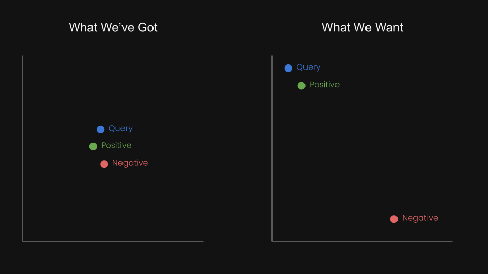
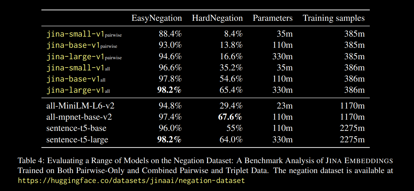
For example, "Flight from Amsterdam to Berlin" could be considered the negative pair of “Flight from Berlin to Amsterdam”. In fact, in the jina-embeddings-v1 technical report (Michael Guenther, et al.), we briefly addressed this issue on a small scale: we fine-tuned the jina-embeddings-v1 model on a negation dataset of 10,000 examples generated from large language models.
The results, reported in the report link above, were promising:
We observe that across all model sizes, fine-tuning on triplet data (which includes our negation training dataset) dramatically enhances performance, particularly on the HardNegation task.
jina-embeddings models with both pairwise and combined triplet/pairwise training.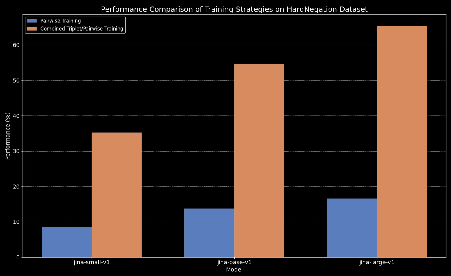
jina-embeddings.tagFine-Tuning Text Embedding Models with Curated Datasets
In the previous sections, we explored several key observations regarding text embeddings:
- Shorter texts are more prone to errors in capturing word order.
- Increasing the size of the text embedding model doesn’t necessarily improve word order understanding.
- Contrastive learning could offer a potential solution to these issues.
With this in mind, we fine-tuned jina-embeddings-v2-base-en and bge-base-en-1.5 on our negation and word ordering datasets (about 11,000 training samples in total):


To help evaluate the fine-tuning, we generated a dataset of 1,000 triplets consisting of a query, positive (pos), and negative (neg) case:
Here’s an example row:
| Anchor | The river flows from the mountains to the sea |
| Positive | Water travels from mountain peaks to ocean |
| Negative | The river flows from the sea to the mountains |
These triplets are designed to cover various failure cases, including directional, temporal, and causal shifts in meaning due to word order changes.
We can now evaluate the models on three different evaluation sets:
- The set of 180 synthetic sentences (from earlier in this post), randomly shuffled.
- Five manually checked examples (from the directional/causal/etc table above).
- 94 curated triplets from our triplet dataset we just generated.
Here’s the difference for shuffled sentences before and after fine-tuning:
| Sentence Length (tokens) | Mean Cosine Similarity (jina) |
Mean Cosine Similarity (jina-ft) |
Mean Cosine Similarity (bge) |
Mean Cosine Similarity (bge-ft) |
|---|---|---|---|---|
| 3 | 0.970 | 0.927 | 0.929 | 0.899 |
| 5 | 0.958 | 0.910 | 0.940 | 0.916 |
| 10 | 0.953 | 0.890 | 0.934 | 0.910 |
| 15 | 0.930 | 0.830 | 0.912 | 0.875 |
| 20 | 0.916 | 0.815 | 0.901 | 0.879 |
| 30 | 0.927 | 0.819 | 0.877 | 0.852 |
The result seems clear: despite the fine-tuning process only taking five minutes, we see dramatic improvement in performance on the dataset of randomly-shuffled sentences:
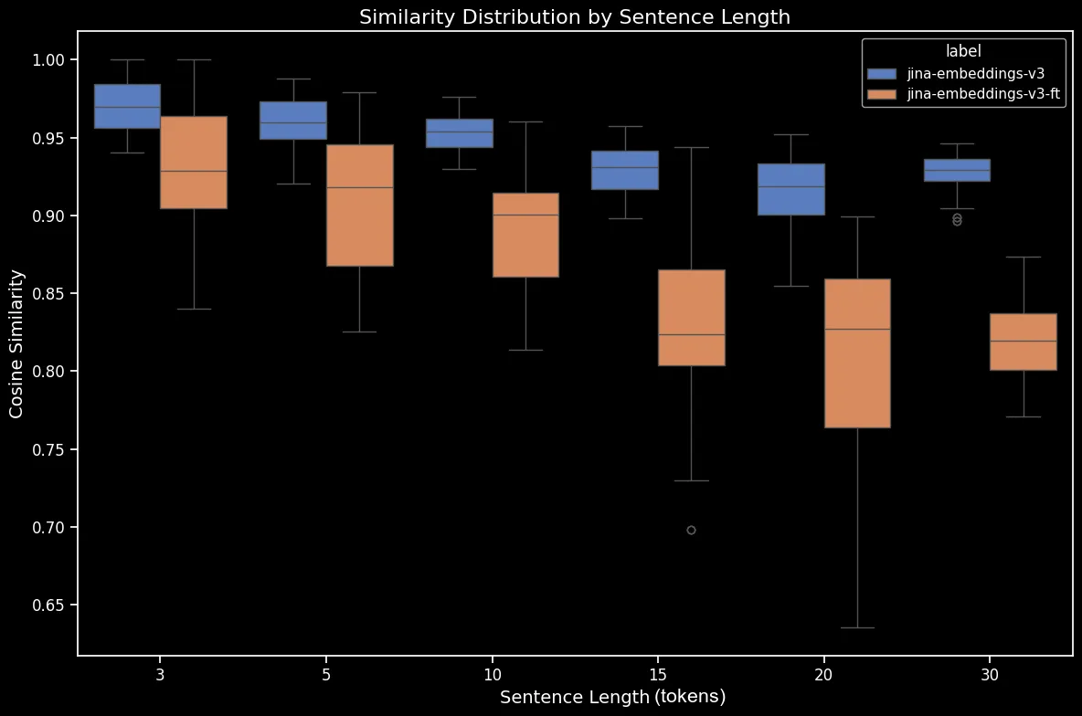
bge-base-en-1.5 (finetuned).We also see gains on directional, temporal, causal and comparative cases. The model shows a substantial performance improvement reflected by a drop of averaged cosine similarity. The biggest performance gain is on the negation case, due to our fine-tuning dataset containing 10,000 negation training examples.
| Category | Example - Left | Example - Right | Mean Cosine Similarity (jina) |
Mean Cosine Similarity (jina-ft) |
Mean Cosine Similarity (bge) |
Mean Cosine Similarity (bge-ft) |
|---|---|---|---|---|---|---|
| Directional | She flew from Paris to Tokyo. | She drove from Tokyo to Paris | 0.9439 | 0.8650 | 0.9319 | 0.8674 |
| Temporal | She ate dinner before watching the movie | She watched the movie before eating dinner | 0.9833 | 0.9263 | 0.9683 | 0.9331 |
| Causal | The rising temperature melted the snow | The melting snow cooled the temperature | 0.8998 | 0.7937 | 0.8874 | 0.8371 |
| Comparative | Coffee tastes better than tea | Tea tastes better than coffee | 0.9457 | 0.8759 | 0.9723 | 0.9030 |
| Negation | He is standing by the table | He is standing far from the table | 0.9116 | 0.4478 | 0.8329 | 0.4329 |
tagConclusion
In this post, we dive into the challenges text embedding models face, especially their struggle to handle word order effectively. To break it down, we’ve identified five main failure types: Directional, Temporal, Causal, Comparative, and Negation. These are the kinds of queries where word order really matters, and if your use case involves any of these, it’s worth knowing the limitations of these models.
We also ran a quick experiment, expanding a negation-focused dataset to cover all five failure categories. The results were promising: fine-tuning with carefully chosen "hard negatives" made the model better at recognizing which items belong together and which don’t. That said, there’s more work to do. Future steps include digging deeper into how the size and quality of the dataset affect performance.


