차세대 클라우드 AI: Amazon SageMaker의 Jina Embeddings와 Rerankers

Jina Embeddings와 Jina Reranker가 이제 AWS Marketplace를 통해 Amazon SageMaker에서 사용할 수 있게 되었습니다. 보안, 신뢰성, 클라우드 운영의 일관성을 중요시하는 기업 사용자들은 이제 Jina AI의 최첨단 AI를 자신들의 private AWS 배포 환경에서 사용할 수 있으며, AWS의 안정적인 인프라의 모든 장점을 누릴 수 있습니다.

AWS Marketplace에서 제공되는 모든 임베딩 및 재순위화 모델을 통해, SageMaker 사용자들은 8k 입력 컨텍스트 윈도우와 최고 수준의 다국어 임베딩을 경쟁력 있는 가격으로 온디맨드로 활용할 수 있습니다. AWS로 모델을 전송하거나 AWS에서 모델을 전송하는 데 비용을 지불할 필요가 없으며, 가격이 투명하고 AWS 계정과 통합된 청구 시스템을 이용할 수 있습니다.

현재 Amazon SageMaker에서 사용 가능한 모델은 다음과 같습니다:

• Jina Embeddings v2 Base - English
• Jina Embeddings v2 Small - English
• Jina Embeddings v2 Bilingual Models:
  • German/English
  • Chinese/English
  • Spanish/English
• Jina Embeddings v2 Base - Code
• Jina Reranker v1 Base - English
• Jina ColBERT v1 - English
• Jina ColBERT Reranker v1 - English

전체 모델 목록은 AWS Marketplace의 Jina AI 벤더 페이지에서 확인할 수 있으며, 7일 무료 평가판을 이용할 수 있습니다.

AWS Marketplace: Jina AI

이 글에서는 Amazon SageMaker의 구성 요소만을 사용하여 Retrieval-augmented generation(RAG) 애플리케이션을 만드는 방법을 안내합니다. 우리가 사용할 모델은 Jina Embeddings v2 - English, Jina Reranker v1, 그리고 Mistral-7B-Instruct 대규모 언어 모델입니다.

Python Notebook을 통해서도 따라할 수 있으며, 다운로드하거나 Google Colab에서 실행할 수 있습니다.

tagRetrieval-Augmented Generation

Retrieval-augmented generation은 생성형 AI의 대안적 패러다임입니다. 대규모 언어 모델(LLM)이 학습한 내용을 바탕으로 사용자 요청에 직접 답변하는 대신, 유창한 언어 생성 능력을 활용하면서 로직과 정보 검색을 더 적합한 외부 장치로 이전합니다.

RAG 시스템은 LLM을 호출하기 전에 외부 데이터 소스에서 관련 정보를 적극적으로 검색하여 프롬프트의 일부로 LLM에 제공합니다. LLM의 역할은 외부 정보를 사용자 요청에 대한 일관된 응답으로 합성하여 환각 위험을 최소화하고 결과의 관련성과 유용성을 높이는 것입니다.

RAG 시스템은 기본적으로 다음 네 가지 구성 요소를 가집니다:

• 일반적으로 AI 지원 정보 검색에 적합한 벡터 데이터베이스와 같은 데이터 소스
• 사용자의 요청을 쿼리로 취급하여 답변에 관련된 데이터를 검색하는 정보 검색 시스템
• AI 기반 재순위화 모델을 포함하여 검색된 데이터 중 일부를 선택하고 LLM용 프롬프트로 처리하는 시스템
• 사용자 요청과 제공된 데이터를 받아 사용자에게 응답을 생성하는 LLM(예: GPT 모델이나 Mistral과 같은 오픈소스 LLM)

임베딩 모델은 정보 검색에 매우 적합하며 이러한 목적으로 자주 사용됩니다. 텍스트 임베딩 모델은 텍스트를 입력으로 받아 임베딩(고차원 벡터)을 출력하는데, 이 임베딩들 간의 공간적 관계가 의미적 유사성(즉, 유사한 주제, 내용 및 관련 의미)을 나타냅니다. 임베딩이 가까울수록 사용자가 응답에 만족할 가능성이 높기 때문에 정보 검색에 자주 사용되며, 특정 도메인에서의 성능을 향상시키기 위해 비교적 쉽게 미세 조정할 수 있습니다.

텍스트 재순위화 모델은 유사한 AI 원리를 사용하여 텍스트 모음을 쿼리와 비교하고 의미적 유사성에 따라 정렬합니다. 임베딩 모델에만 의존하는 대신 작업별 재순위화 모델을 사용하면 검색 결과의 정확도가 크게 향상되는 경우가 많습니다. RAG 애플리케이션의 재순위화 모델은 LLM 프롬프트에 올바른 정보가 포함될 확률을 최대화하기 위해 정보 검색 결과 중 일부를 선택합니다.

Maximizing Search Relevance and RAG Accuracy with Jina Reranker

Boost your search and RAG accuracy with Jina Reranker. Our new model improves the accuracy and relevance by 20% over simple vector search. Try it now for free!

tagSageMaker 엔드포인트로서의 임베딩 모델 성능 벤치마킹

우리는 Jina Embeddings v2 Base - English 모델의 SageMaker 엔드포인트 성능과 신뢰성을 g4dn.xlarge 인스턴스에서 테스트했습니다. 이 실험에서는 매초마다 새로운 사용자를 지속적으로 생성하여, 각 사용자가 요청을 보내고 응답을 기다린 후 응답을 받으면 반복하도록 했습니다.

• 100 토큰 미만의 요청의 경우, 최대 150명의 동시 사용자까지는 요청당 응답 시간이 100ms 미만으로 유지되었습니다. 이후 동시 사용자가 증가함에 따라 응답 시간이 100ms에서 1500ms까지 선형적으로 증가했습니다.
  • 약 300명의 동시 사용자에서 API에서 5회 이상의 실패가 발생하여 테스트를 종료했습니다.
• 1K에서 8K 토큰 사이의 요청의 경우, 최대 20명의 동시 사용자까지는 요청당 응답 시간이 8초 미만으로 유지되었습니다. 이후 동시 사용자가 증가함에 따라 응답 시간이 8초에서 60초까지 선형적으로 증가했습니다.
  • 약 140명의 동시 사용자에서 API에서 5회 이상의 실패가 발생하여 테스트를 종료했습니다.

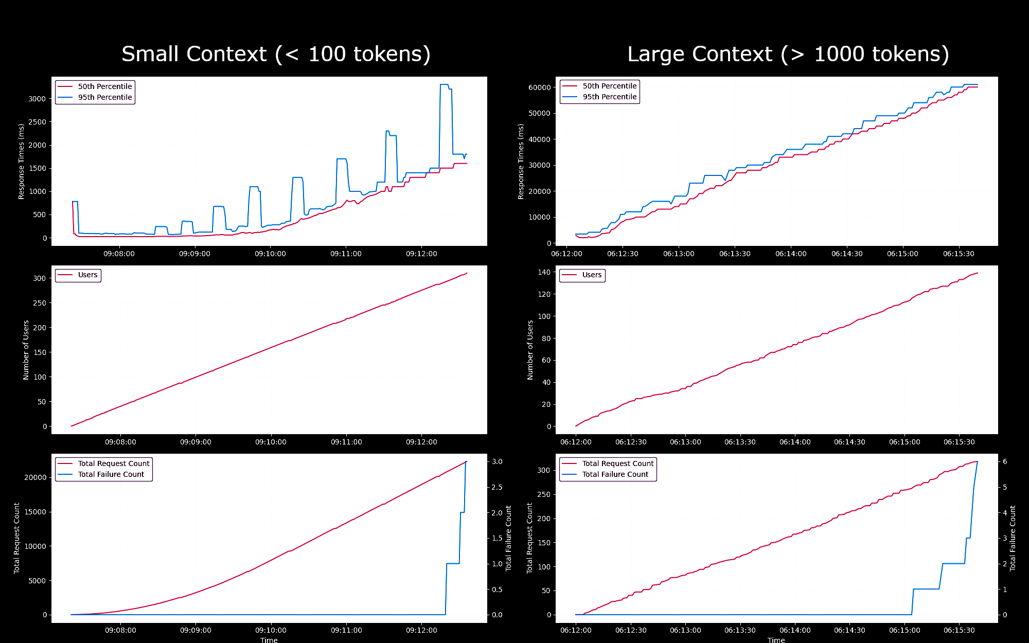
이러한 결과를 바탕으로, 일반적인 임베딩 워크로드를 가진 대부분의 사용자에게는 g4dn.xlarge 또는 g5.xlarge 인스턴스가 일상적인 요구를 충족시킬 수 있다고 결론 내릴 수 있습니다. 하지만 검색 작업보다 훨씬 덜 자주 실행되는 대규모 인덱싱 작업의 경우, 사용자들은 더 높은 성능의 옵션을 선호할 수 있습니다. 사용 가능한 모든 Sagemaker 인스턴스 목록은 AWS의 EC2 개요를 참조하세요.

tagAWS 계정 구성하기

먼저, AWS 계정이 필요합니다. 아직 AWS 사용자가 아니라면, AWS 웹사이트에서 계정에 가입할 수 있습니다.

AWS Console - Signup

Signup

tagPython 환경에서 AWS 도구 설정하기

이 튜토리얼에 필요한 AWS 도구와 라이브러리를 Python 환경에 설치하세요:

pip install awscli jina-sagemaker
Copy

AWS 계정의 액세스 키와 시크릿 액세스 키가 필요합니다. AWS 웹사이트의 지침에 따라 이를 얻을 수 있습니다.

Managing access keys for IAM users - AWS Identity and Access Management

Create, modify, view, or update access keys (credentials) for programmatic calls to AWS.

AWS Identity and Access Management

또한 작업할 AWS 리전을 선택해야 합니다.

Regions, Availability Zones, and Local Zones - Amazon Relational Database Service

Learn how Amazon cloud computing resources are hosted in multiple locations world-wide, including AWS Regions and Availability Zones.

Amazon Relational Database Service

그런 다음 환경 변수에 값을 설정하세요. Python 또는 Python 노트북에서는 다음 코드로 설정할 수 있습니다:

import os

os.environ["AWS_ACCESS_KEY_ID"] = <YOUR_ACCESS_KEY_ID>
os.environ["AWS_SECRET_ACCESS_KEY"] = <YOUR_SECRET_ACCESS_KEY>
os.environ["AWS_DEFAULT_REGION"] = <YOUR_AWS_REGION>
os.environ["AWS_DEFAULT_OUTPUT"] = "json"
Copy

기본 출력을 json으로 설정하세요.

이는 AWS 명령줄 애플리케이션을 통해서나 로컬 파일시스템에 AWS 구성 파일을 설정하여 수행할 수도 있습니다. 자세한 내용은 AWS 웹사이트의 문서를 참조하세요.

tag역할 생성하기

이 튜토리얼에 필요한 리소스를 사용하기 위해 충분한 권한을 가진 AWS 역할도 필요합니다.

이 역할은 다음을 갖추어야 합니다:

1. AmazonSageMakerFullAccess가 활성화되어 있어야 함
2. 다음 중 하나:
   1. AWS Marketplace 구독을 할 수 있는 권한이 있고 다음 세 가지가 모두 활성화되어 있어야 함:
      1. aws-marketplace:ViewSubscriptions
      2. aws-marketplace:Unsubscribe
      3. aws-marketplace:Subscribe
   2. 또는 AWS 계정이 jina-embedding-model을 구독하고 있어야 함

역할의 ARN(Amazon Resource Name)을 role 변수에 저장하세요:

role = <YOUR_ROLE_ARN>
Copy

자세한 내용은 AWS 웹사이트의 역할 관련 문서를 참조하세요.

IAM roles - AWS Identity and Access Management

Learn how and when to use IAM roles.

AWS Identity and Access Management

tagAWS Marketplace에서 Jina AI 모델 구독하기

이 글에서는 Jina Embeddings v2 base English 모델을 사용할 것입니다. AWS Marketplace에서 이를 구독하세요.

AWS Marketplace: Jina Embeddings v2 Base - en

en

페이지를 아래로 스크롤하면 가격 정보를 볼 수 있습니다. AWS는 마켓플레이스의 모델에 대해 시간당 요금을 부과하므로, 모델 엔드포인트를 시작한 시점부터 중지할 때까지의 시간에 대해 청구됩니다. 이 글에서는 두 가지 방법 모두를 보여드릴 것입니다.

또한 구독이 필요한 Jina Reranker v1 - English 모델도 사용할 것입니다.

AWS Marketplace: Jina Reranker v1 Base - en

en

구독하신 후에는 AWS 리전에 대한 모델의 ARN을 얻어서 embedding_package_arn과 reranker_package_arn 변수 이름으로 저장하시면 됩니다. 이 튜토리얼의 코드는 이러한 변수 이름을 참조할 것입니다.

ARN을 얻는 방법을 모르시는 경우, Amazon 리전 이름을 region 변수에 넣고 다음 코드를 사용하세요:

region = os.environ["AWS_DEFAULT_REGION"]

def get_arn_for_model(region_name, model_name):
    model_package_map = {
        "us-east-1": f"arn:aws:sagemaker:us-east-1:253352124568:model-package/{model_name}",
        "us-east-2": f"arn:aws:sagemaker:us-east-2:057799348421:model-package/{model_name}",
        "us-west-1": f"arn:aws:sagemaker:us-west-1:382657785993:model-package/{model_name}",
        "us-west-2": f"arn:aws:sagemaker:us-west-2:594846645681:model-package/{model_name}",
        "ca-central-1": f"arn:aws:sagemaker:ca-central-1:470592106596:model-package/{model_name}",
        "eu-central-1": f"arn:aws:sagemaker:eu-central-1:446921602837:model-package/{model_name}",
        "eu-west-1": f"arn:aws:sagemaker:eu-west-1:985815980388:model-package/{model_name}",
        "eu-west-2": f"arn:aws:sagemaker:eu-west-2:856760150666:model-package/{model_name}",
        "eu-west-3": f"arn:aws:sagemaker:eu-west-3:843114510376:model-package/{model_name}",
        "eu-north-1": f"arn:aws:sagemaker:eu-north-1:136758871317:model-package/{model_name}",
        "ap-southeast-1": f"arn:aws:sagemaker:ap-southeast-1:192199979996:model-package/{model_name}",
        "ap-southeast-2": f"arn:aws:sagemaker:ap-southeast-2:666831318237:model-package/{model_name}",
        "ap-northeast-2": f"arn:aws:sagemaker:ap-northeast-2:745090734665:model-package/{model_name}",
        "ap-northeast-1": f"arn:aws:sagemaker:ap-northeast-1:977537786026:model-package/{model_name}",
        "ap-south-1": f"arn:aws:sagemaker:ap-south-1:077584701553:model-package/{model_name}",
        "sa-east-1": f"arn:aws:sagemaker:sa-east-1:270155090741:model-package/{model_name}",
    }

    return model_package_map[region_name]

embedding_package_arn = get_arn_for_model(region, "jina-embeddings-v2-base-en")
reranker_package_arn = get_arn_for_model(region, "jina-reranker-v1-base-en")
Copy

tag데이터셋 로드하기

이 튜토리얼에서는 YouTube 채널 TU Delft Online Learning에서 제공하는 비디오 컬렉션을 사용할 것입니다. 이 채널은 STEM 과목에 대한 다양한 교육 자료를 제작합니다. 프로그래밍은 CC-BY 라이선스를 따릅니다.

TU Delft Online Learning

과학, 디자인 또는 엔지니어링 분야에서 경력을 쌓고 싶으신가요? 그렇다면 TU Delft의 온라인 학습자 커뮤니티에 참여하세요! TU Delft에서 온라인 학습은 능동적 학습을 의미합니다. 우리의 강좌들은 여러분에게 매력적인 학습 경험을 제공하도록 설계되었습니다. 강좌 내용은 도전적이고 까다로우며, 개인적 성장과 전문성 개발을 촉진하면서도 온라인 강좌가 제공하는 유연성과 접근성을 통해 삶의 다른 우선순위들과 학습을 병행할 수 있도록 합니다. 오늘 학습을 시작하세요: https://online-learning.tud…

YouTube

우리는 이 채널에서 193개의 비디오를 다운로드하여 OpenAI의 오픈소스 Whisper 음성 인식 모델로 처리했습니다. 가장 작은 모델인 openai/whisper-tiny를 사용하여 비디오를 텍스트로 변환했습니다.

변환된 텍스트는 CSV 파일로 정리되어 있으며, 여기서 다운로드할 수 있습니다.

파일의 각 행에는 다음이 포함되어 있습니다:

• 비디오 제목
• YouTube 비디오 URL
• 비디오의 텍스트 변환본

Python에서 이 데이터를 로드하려면 먼저 pandas와 requests를 설치하세요:

pip install requests pandas
Copy

CSV 데이터를 직접 tu_delft_dataframe이라는 Pandas DataFrame으로 로드하세요:

import pandas

# Load the CSV file
tu_delft_dataframe = pandas.read_csv("https://raw.githubusercontent.com/jina-ai/workshops/feat-sagemaker-post/notebooks/embeddings/sagemaker/tu_delft.csv")
Copy

DataFrame의 head() 메서드를 사용하여 내용을 확인할 수 있습니다. 노트북에서는 다음과 같이 표시될 것입니다:

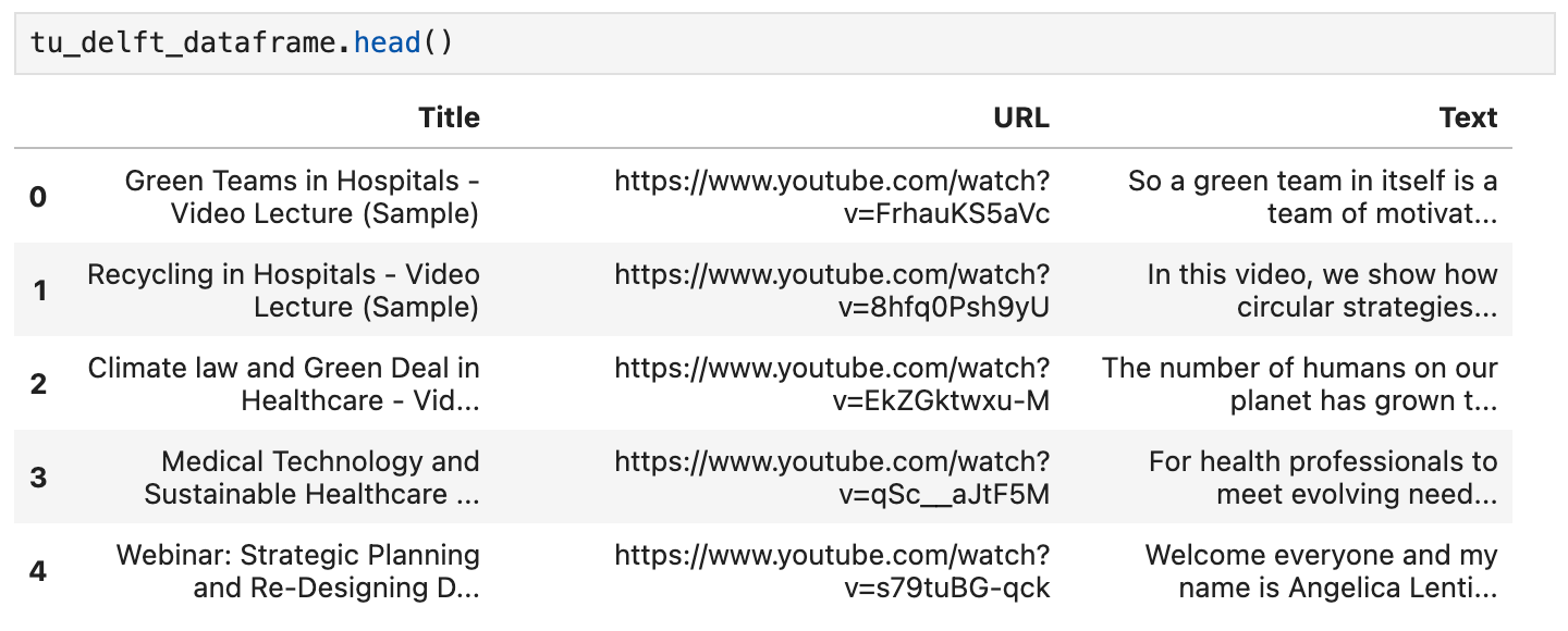
이 데이터셋에 주어진 URL을 사용하여 비디오를 시청할 수도 있으며, 음성 인식이 완벽하지는 않지만 기본적으로 정확하다는 것을 확인할 수 있습니다.

tagJina Embeddings v2 엔드포인트 시작하기

아래 코드는 임베딩 모델을 실행하기 위해 AWS에서 ml.g4dn.xlarge 인스턴스를 시작할 것입니다. 이 작업이 완료되는 데 몇 분이 걸릴 수 있습니다.

import boto3
from jina_sagemaker import Client

# Choose a name for your embedding endpoint. It can be anything convenient.
embeddings_endpoint_name = "jina_embedding"

embedding_client = Client(region_name=boto3.Session().region_name)
embedding_client.create_endpoint(
    arn=embedding_package_arn,
    role=role,
    endpoint_name=embeddings_endpoint_name,
    instance_type="ml.g4dn.xlarge",
    n_instances=1,
)

embedding_client.connect_to_endpoint(endpoint_name=embeddings_endpoint_name)
Copy

필요한 경우 instance_type을 변경하여 다른 AWS 클라우드 인스턴스 유형을 선택할 수 있습니다.

tag데이터셋 구축 및 인덱싱

이제 데이터를 로드하고 Jina Embeddings v2 모델을 실행하고 있으므로, 데이터를 준비하고 인덱싱할 수 있습니다. 데이터는 AI 애플리케이션을 위해 특별히 설계된 오픈소스 벡터 데이터베이스인 FAISS 벡터 스토어에 저장할 것입니다.

먼저 RAG 애플리케이션에 필요한 나머지 필수 패키지들을 설치하세요:

pip install tdqm numpy faiss-cpu
Copy

tag청킹

LLM의 프롬프트에 여러 텍스트를 맞출 수 있도록 개별 텍스트를 더 작은 부분, 즉 "청크"로 나눌 필요가 있습니다. 아래 코드는 문장 경계를 기준으로 개별 텍스트를 나누며, 기본적으로 모든 청크가 128단어를 넘지 않도록 합니다.

Note: The code blocks below retain their original English/code content as per translation guidelines.

def chunk_text(text, max_words=128):
    """
    Divide text into chunks where each chunk contains the maximum number 
    of full sentences with fewer words than `max_words`.
    """
    sentences = text.split(".")
    chunk = []
    word_count = 0

    for sentence in sentences:
        sentence = sentence.strip(".")
        if not sentence:
          continue

        words_in_sentence = len(sentence.split())
        if word_count + words_in_sentence <= max_words:
            chunk.append(sentence)
            word_count += words_in_sentence
        else:
            # Yield the current chunk and start a new one
            if chunk:
              yield ". ".join(chunk).strip() + "."
            chunk = [sentence]
            word_count = words_in_sentence

    # Yield the last chunk if it's not empty
    if chunk:
        yield " ".join(chunk).strip() + "."
Copy

tag각 청크의 임베딩 가져오기

FAISS 데이터베이스에 저장하기 위해 각 청크의 임베딩이 필요합니다. 이를 위해 텍스트 청크를 Jina AI 임베딩 모델 엔드포인트에 embedding_client.embed() 메서드를 사용하여 전달합니다. 그런 다음 텍스트 청크와 임베딩 벡터를 pandas 데이터프레임 tu_delft_dataframe에 chunks와 embeddings라는 새로운 열로 추가합니다:

import numpy as np
from tqdm import tqdm

tqdm.pandas()

def generate_embeddings(text_df):
    chunks = list(chunk_text(text_df["Text"]))
    embeddings = []

    for i, chunk in enumerate(chunks):
      response = embedding_client.embed(texts=[chunk])
      chunk_embedding = response[0]["embedding"]
      embeddings.append(np.array(chunk_embedding))

    text_df["chunks"] = chunks
    text_df["embeddings"] = embeddings
    return text_df

print("Embedding text chunks ...")
tu_delft_dataframe = generate_embeddings(tu_delft_dataframe)
## Google Colab이나 Python 노트북을 사용하는 경우
## 위 줄을 삭제하고 다음 줄의 주석을 해제하세요:
# tu_delft_dataframe = tu_delft_dataframe.progress_apply(generate_embeddings, axis=1)
Copy

tagFaiss를 사용한 의미 검색 설정

아래 코드는 FAISS 데이터베이스를 생성하고 tu_delft_pandas를 반복하여 청크와 임베딩 벡터를 삽입합니다:

import faiss

dim = 768  # Jina v2 임베딩의 차원
index_with_ids = faiss.IndexIDMap(faiss.IndexFlatIP(dim))
k = 0

doc_ref = dict()

for idx, row in tu_delft_dataframe.iterrows():
    embeddings = row["embeddings"]
    for i, embedding in enumerate(embeddings):
        normalized_embedding = np.ascontiguousarray(np.array(embedding, dtype="float32").reshape(1, -1))
        faiss.normalize_L2(normalized_embedding)
        index_with_ids.add_with_ids(normalized_embedding, k)
        doc_ref[k] = (row["chunks"][i], idx)
        k += 1
Copy

tagJina Reranker v1 엔드포인트 시작

위의 Jina Embedding v2 모델과 마찬가지로, 이 코드는 AWS에서 리랭커 모델을 실행하기 위해 ml.g4dn.xlarge 인스턴스를 시작합니다. 마찬가지로 실행하는 데 몇 분이 걸릴 수 있습니다.

import boto3
from jina_sagemaker import Client

# 리랭커 엔드포인트의 이름을 선택하세요. 편리한 이름이면 됩니다.
reranker_endpoint_name = "jina_reranker"

reranker_client = Client(region_name=boto3.Session().region_name)
reranker_client.create_endpoint(
    arn=reranker_package_arn,
    role=role,
    endpoint_name=reranker_endpoint_name,
    instance_type="ml.g4dn.xlarge",
    n_instances=1,
)

reranker_client.connect_to_endpoint(endpoint_name=reranker_endpoint_name)
Copy

tag쿼리 함수 정의

다음으로, 텍스트 쿼리와 가장 유사한 트랜스크립트 청크를 식별하는 함수를 정의하겠습니다.

이는 두 단계로 이루어진 프로세스입니다:

1. 데이터 준비 단계에서처럼 embedding_client.embed() 메서드를 사용하여 사용자 입력을 임베딩 벡터로 변환합니다.
2. 임베딩을 FAISS 인덱스에 전달하여 가장 잘 매치되는 결과를 검색합니다. 아래 함수에서는 기본값으로 상위 20개의 매치를 반환하지만, n 매개변수로 이를 제어할 수 있습니다.

find_most_similar_transcript_segment 함수는 저장된 임베딩과 쿼리 임베딩의 코사인을 비교하여 가장 적합한 매치를 반환합니다.

def find_most_similar_transcript_segment(query, n=20):
    query_embedding = embedding_client.embed(texts=[query])[0]["embedding"]  # Assuming the query is short enough to not need chunking
    query_embedding = np.ascontiguousarray(np.array(query_embedding, dtype="float32").reshape(1, -1))
    faiss.normalize_L2(query_embedding)

    D, I = index_with_ids.search(query_embedding, n)  # Get the top n matches

    results = []
    for i in range(n):
        distance = D[0][i]
        index_id = I[0][i]
        transcript_segment, doc_idx = doc_ref[index_id]
        results.append((transcript_segment, doc_idx, distance))

    # Sort the results by distance
    results.sort(key=lambda x: x[2])

    return [(tu_delft_dataframe.iloc[r[1]]["Title"].strip(), r[0]) for r in results]
Copy

또한 리랭커 엔드포인트 reranker_client에 접근하여 find_most_similar_transcript_segment의 결과를 전달하고 가장 관련성 높은 3개의 결과만 반환하는 함수를 정의할 것입니다. 이는 reranker_client.rerank() 메서드로 리랭커 엔드포인트를 호출합니다.

def rerank_results(query_found, query, n=3):
    ret = reranker_client.rerank(
        documents=[f[1] for f in query_found], 
        query=query, 
        top_n=n,
    )
    return [query_found[r['index']] for r in ret[0]['results']]
Copy

tagJumpStart를 사용하여 Mistral-Instruct 로드하기

이 튜토리얼에서는 RAG 시스템의 LLM 부분으로 mistral-7b-instruct 모델을 사용할 것입니다. 이 모델은 Amazon SageMaker JumpStart를 통해 사용 가능합니다.

Mistral 7B foundation models from Mistral AI are now available in Amazon SageMaker JumpStart | Amazon Web Services

Today, we are excited to announce that the Mistral 7B foundation models, developed by Mistral AI, are available for customers through Amazon SageMaker JumpStart to deploy with one click for running inference. With 7 billion parameters, Mistral 7B can be easily customized and quickly deployed. You can try out this model with SageMaker JumpStart, a […]

Amazon Web Services

Mistral-Instruct를 로드하고 배포하기 위해 다음 코드를 실행하세요:

from sagemaker.jumpstart.model import JumpStartModel

jumpstart_model = JumpStartModel(model_id="huggingface-llm-mistral-7b-instruct", role=role)
model_predictor = jumpstart_model.deploy()
Copy

이 LLM에 접근하기 위한 엔드포인트는 model_predictor 변수에 저장됩니다.

tagJumpStart의 Mistral-Instruct

아래는 Python의 내장 문자열 템플릿 클래스를 사용하여 이 애플리케이션을 위한 Mistral-Instruct의 프롬프트 템플릿을 만드는 코드입니다. 각 쿼리마다 모델에 제시될 세 개의 매칭되는 트랜스크립트 청크가 있다고 가정합니다.

이 템플릿을 직접 실험하여 이 애플리케이션을 수정하거나 더 나은 결과를 얻을 수 있는지 확인해 볼 수 있습니다.

from string import Template

prompt_template = Template("""
  <s>[INST] Answer the question below only using the given context.
  The question from the user is based on transcripts of videos from a YouTube
    channel.
  The context is presented as a ranked list of information in the form of
    (video-title, transcript-segment), that is relevant for answering the
    user's question.
  The answer should only use the presented context. If the question cannot be
    answered based on the context, say so.

  Context:
  1. Video-title: $title_1, transcript-segment: $segment_1
  2. Video-title: $title_2, transcript-segment: $segment_2
  3. Video-title: $title_3, transcript-segment: $segment_3

  Question: $question

  Answer: [/INST]
""")
Copy

이 구성 요소가 준비되면 이제 완전한 RAG 애플리케이션의 모든 부분이 갖춰졌습니다.

tag모델 쿼리하기

모델 쿼리는 세 단계로 이루어진 프로세스입니다.

1. 쿼리가 주어졌을 때 관련 청크를 검색합니다.
2. 프롬프트를 구성합니다.
3. 프롬프트를 Mistral-Instruct 모델에 전송하고 답변을 반환합니다.

관련 청크를 검색하기 위해 위에서 정의한 find_most_similar_transcript_segment 함수를 사용합니다.

question = "When was the first offshore wind farm commissioned?"
search_results = find_most_similar_transcript_segment(question)
reranked_results = rerank_results(search_results, question)
Copy

검색 결과를 재순위화된 순서로 확인할 수 있습니다:

for title, text, _ in reranked_results:
    print(title + "\n" + text + "\n")
Copy

결과:

Offshore Wind Farm Technology - Course Introduction
Since the first offshore wind farm commissioned in 1991 in Denmark, scientists and engineers have adapted and improved the technology of wind energy to offshore conditions.  This is a rapidly evolving field with installation of increasingly larger wind turbines in deeper waters.  At sea, the challenges are indeed numerous, with combined wind and wave loads, reduced accessibility and uncertain-solid conditions.  My name is Axel Vire, I'm an assistant professor in Wind Energy at U-Delf and specializing in offshore wind energy.  This course will touch upon the critical aspect of wind energy, how to integrate the various engineering disciplines involved in offshore wind energy.  Each week we will focus on a particular discipline and use it to design and operate a wind farm.

Offshore Wind Farm Technology - Course Introduction
I'm a researcher and lecturer at the Wind Energy and Economics Department and I will be your moderator throughout this course.  That means I will answer any questions you may have.  I'll strengthen the interactions between the participants and also I'll get you in touch with the lecturers when needed.  The course is mainly developed for professionals in the field of offshore wind energy.  We want to broaden their knowledge of the relevant technical disciplines and their integration.  Professionals with a scientific background who are new to the field of offshore wind energy will benefit from a high-level insight into the engineering aspects of wind energy.  Overall, the course will help you make the right choices during the development and operation of offshore wind farms.

Offshore Wind Farm Technology - Course Introduction
Designed wind turbines that better withstand wind, wave and current loads  Identify great integration strategies for offshore wind turbines and gain understanding of the operational and maintenance of offshore wind turbines and farms  We also hope that you will benefit from the course and from interaction with other learners who share your interest in wind energy  And therefore we look forward to meeting you online.
Copy

이 정보를 프롬프트 템플릿에 직접 사용할 수 있습니다:

prompt_for_llm = prompt_template.substitute(
    question = question,
    title_1 = search_results[0][0],
    segment_1 = search_results[0][1],
    title_2 = search_results[1][0],
    segment_2 = search_results[1][1],
    title_3 = search_results[2][0],
    segment_3 = search_results[2][1],
)
Copy

LLM에 실제로 전송되는 프롬프트를 확인하기 위해 결과 문자열을 출력합니다:

print(prompt_for_llm)
Copy

<s>[INST] Answer the question below only using the given context.
  The question from the user is based on transcripts of videos from a YouTube
    channel.
  The context is presented as a ranked list of information in the form of
    (video-title, transcript-segment), that is relevant for answering the
    user's question.
  The answer should only use the presented context. If the question cannot be
    answered based on the context, say so.

  Context:
  1. Video-title: Offshore Wind Farm Technology - Course Introduction, transcript-segment: Since the first offshore wind farm commissioned in 1991 in Denmark, scientists and engineers have adapted and improved the technology of wind energy to offshore conditions.  This is a rapidly evolving field with installation of increasingly larger wind turbines in deeper waters.  At sea, the challenges are indeed numerous, with combined wind and wave loads, reduced accessibility and uncertain-solid conditions.  My name is Axel Vire, I'm an assistant professor in Wind Energy at U-Delf and specializing in offshore wind energy.  This course will touch upon the critical aspect of wind energy, how to integrate the various engineering disciplines involved in offshore wind energy.  Each week we will focus on a particular discipline and use it to design and operate a wind farm.
  2. Video-title: Offshore Wind Farm Technology - Course Introduction, transcript-segment: For example, we look at how to characterize the wind and wave conditions at a given location.  How to best place the wind turbines in a farm and also how to retrieve the electricity back to shore.  We look at the main design drivers for offshore wind turbines and their components.  We'll see how these aspects influence one another and the best choices to reduce the cost of energy.  This course is organized by the two-delfd wind energy institute, an interfaculty research organization focusing specifically on wind energy.  You will therefore benefit from the expertise of the lecturers in three different faculties of the university.  Aerospace engineering, civil engineering and electrical engineering.  Hi, my name is Ricardo Pareda.
  3. Video-title: Systems Analysis for Problem Structuring part 1B the mono actor perspective example, transcript-segment: So let's assume the demarcation of the problem and the analysis of objectives has led to the identification of three criteria.  The security of supply, the percentage of offshore power generation and the costs of energy provision.  We now reason backwards to explore what factors have an influence on these system outcomes.  Really, the offshore percentage is positively influenced by the installed Wind Power capacity at sea, a key system factor.  Capacity at sea in turn is determined by both the size and the number of wind farms at sea.  The Ministry of Economic Affairs cannot itself invest in new wind farms but hopes to simulate investors and energy companies by providing subsidies and by expediting the granting process of licenses as needed.

  Question: When was the first offshore wind farm commissioned?

  Answer: [/INST]
Copy

이 프롬프트를 model_predictor 메서드 model_predictor.predict()를 통해 LLM 엔드포인트에 전달합니다:

answer = model_predictor.predict({"inputs": prompt_for_llm})
Copy

이는 리스트를 반환하지만, 하나의 프롬프트만 전달했으므로 하나의 항목만 있는 리스트가 됩니다. 각 항목은 generated_text 키 아래에 응답 텍스트가 있는 dict입니다:

answer = answer[0]['generated_text']
print(answer)
Copy

결과:

The first offshore wind farm was commissioned in 1991. (Context: Video-title: Offshore Wind Farm Technology - Course Introduction, transcript-segment: Since the first offshore wind farm commissioned in 1991 in Denmark, ...)
Copy

문자열 질문을 매개변수로 받아 답변을 문자열로 반환하는 함수를 작성하여 쿼리를 단순화해 보겠습니다:

def ask_rag(question):
    search_results = find_most_similar_transcript_segment(question)
    reranked_results = rerank_results(search_results, question)
    prompt_for_llm = prompt_template.substitute(
        question = question,
        title_1 = search_results[0][0],
        segment_1 = search_results[0][1],
        title_2 = search_results[1][0],
        segment_2 = search_results[1][1],
        title_3 = search_results[2][0],
        segment_3 = search_results[2][1],
    )
    answer = model_predictor.predict({"inputs": prompt_for_llm})
    return answer[0]["generated_text"]
Copy

이제 몇 가지 질문을 더 해볼 수 있습니다. 답변은 비디오 트랜스크립트의 내용에 따라 달라집니다. 예를 들어, 데이터에 답이 있는 경우 자세한 질문을 할 수 있습니다:

ask_rag("What is a Kaplan Meyer estimator?")
Copy

The Kaplan Meyer estimator is a non-parametric estimator for the survival 
function, defined for both censored and not censored data. It is represented 
as a series of declining horizontal steps that approaches the truths of the 
survival function if the sample size is sufficiently large enough. The value 
of the empirical survival function obtained is assumed to be constant between 
two successive distinct observations.
Copy

ask_rag("Who is Reneville Solingen?")
Copy

Reneville Solingen is a professor at Delft University of Technology in Global 
Software Engineering. She is also a co-author of the book "The Power of Scrum."
Copy

answer = ask_rag("What is the European Green Deal?")
print(answer)
Copy

The European Green Deal is a policy initiative by the European Union to combat 
climate change and decarbonize the economy, with a goal to make Europe carbon 
neutral by 2050. It involves the use of green procurement strategies in various 
sectors, including healthcare, to reduce carbon emissions and promote corporate 
social responsibility.
Copy

또한 사용 가능한 정보의 범위를 벗어나는 질문도 할 수 있습니다:

ask_rag("What countries export the most coffee?")
Copy

Based on the context provided, there is no clear answer to the user's 
question about which countries export the most coffee as the context 
only discusses the Delft University's cafeteria discounts and sustainable 
coffee options, as well as lithium production and alternatives for use in 
electric car batteries.
Copy

ask_rag("How much wood could a woodchuck chuck if a woodchuck could chuck wood?")
Copy

The context does not provide sufficient information to answer the question. 
The context is about thermit welding of rails, stress concentration factors, 
and a lyrics video. There is no mention of woodchucks or the ability of 
woodchuck to chuck wood in the context.
Copy

직접 쿼리를 시도해보세요. 또한 결과를 개선하기 위해 LLM 프롬프트 방식을 변경할 수도 있습니다.

tag종료하기

사용하는 모델과 AWS 인프라에 대해 시간당 요금이 청구되므로, 이 튜토리얼을 마치면 세 가지 AI 모델을 모두 중지하는 것이 매우 중요합니다:

• 임베딩 모델 엔드포인트 embedding_client
• 재순위화 모델 엔드포인트 reranker_client
• 대규모 언어 모델 엔드포인트 model_predictor

세 가지 모델 엔드포인트를 모두 종료하려면 다음 코드를 실행하세요:

# shut down the embedding endpoint
embedding_client.delete_endpoint()
embedding_client.close()
# shut down the reranker endpoint
reranker_client.delete_endpoint()
reranker_client.close()
# shut down the LLM endpoint
model_predictor.delete_model()
model_predictor.delete_endpoint()
Copy

tagAWS Marketplace에서 Jina AI 모델로 시작하세요

SageMaker의 임베딩 및 재순위화 모델을 통해 AWS의 엔터프라이즈 AI 사용자는 이제 기존 클라우드 운영의 이점을 훼손하지 않고 Jina AI의 뛰어난 가치 제안에 즉시 접근할 수 있습니다. AWS의 모든 보안, 신뢰성, 일관성 및 예측 가능한 가격이 기본으로 제공됩니다.

Jina AI에서는 기존 프로세스에 AI를 도입하여 혜택을 얻을 수 있는 기업에 최첨단 기술을 제공하기 위해 노력하고 있습니다. 우리는 AI에 대한 투자를 최소화하고 수익을 극대화하면서, 편리하고 실용적인 인터페이스를 통해 합리적인 가격으로 안정적이고 고성능의 모델을 제공하기 위해 노력합니다.

우리가 제공하는 모든 임베딩 및 재순위화 모델 목록을 보고 7일 동안 무료로 시험해보려면 Jina AI의 AWS Marketplace 페이지를 확인하세요.

AWS Marketplace: Jina AI

여러분의 사용 사례를 듣고 Jina AI의 제품이 비즈니스 요구사항에 어떻게 부합하는지 논의하고 싶습니다. 웹사이트나 Discord 채널을 통해 연락하시어 피드백을 공유하고 최신 모델 소식을 받아보세요.